Technical Tuesdays: Exploration workflows in Target for ArcGIS Pro

Seequent’s Technical Analyst, Lee Steven, will demonstrate how to:

• Import, visualize and interpret drilling data from standard industry data sources or generic formats
• View drillhole data by numeric or categorical attributes in 2D maps and 3D scenes
• Create cross sections to view and interpret your geology in 3D
• Incorporate subsurface datasets to your project for increased understanding and geological context
• Share and collaborate using Esri’s online workflows and Geospatial Cloud offerings.

Overview

Video Transcript

[00:00:03.910]<v Lee Steven>Hello, and welcome to the “Technical Tuesday”</v>

[00:00:06.220]webinar series.

[00:00:07.300]My name is Lee Steven,

[00:00:08.710]and I’m a Technical Analyst with Seequent Australia.

[00:00:12.390]Today’s webinar topic is

[00:00:13.787]“Exploration Workflows and Target for ArcGIS Pro.”

[00:00:17.440]And we’re going to focus on some of the cornerstones

[00:00:19.740]for surface and drillhole mapping.

[00:00:24.520]The Seequent Solutions encompass

[00:00:25.950]a range of software products.

[00:00:27.360]It’s likable for use across the mining value chain.

[00:00:30.670]As I mentioned in the title,

[00:00:31.730]today, we’re going to focus on Target,

[00:00:33.600]but if you’d like any information

[00:00:35.030]about any of the other software products,

[00:00:37.610]please contact our sales or support staff.

[00:00:43.160]Right now, you can also sign up

[00:00:44.620]for a free 60 day trial of Target for ArcGIS Pro,

[00:00:48.360]and you can do so by registering

[00:00:50.440]through our website at seequent.com.

[00:00:56.420]So in today’s session,

[00:00:57.650]we’re going to do some geophysical data integration

[00:01:00.840]and geochemical data analysis,

[00:01:03.380]some drillhole plotting in 2D maps and 3D scenes.

[00:01:07.240]We’re going to import some 3D models

[00:01:09.160]and display it with the rest of our subsurface data,

[00:01:12.550]create some cross-sections,

[00:01:14.910]plan some new drillholes

[00:01:16.670]and then we’ll wrap up with some tools

[00:01:18.130]for sharing your projects.

[00:01:22.650]If you don’t know what Target for ArcGIS Pro is,

[00:01:24.970]it’s a software extension

[00:01:27.030]that enables you to easily import,

[00:01:30.120]visualize and interpret your drillhole

[00:01:32.100]and geologic datasets in ArcGIS Pro.

[00:01:37.150]There’s also a number of free tools available in Target.

[00:01:40.010]We’ve got some tools for importing 2D grids, 3D models,

[00:01:45.240]searching and download public domain data sets

[00:01:48.040]through our geoscience data portals,

[00:01:51.140]some tools for enhancing Greta data,

[00:01:54.200]as well as some tools

[00:01:55.410]for helping you navigate the 3D scenes.

[00:02:00.700]I’m now going to jump into ArcGIS Pro

[00:02:02.630]for the live demonstration portion.

[00:02:07.770]And so our project begins

[00:02:09.040]in Southeast British Columbia in Canada.

[00:02:12.440]In the early stages of the project,

[00:02:13.890]historical data were reviewed

[00:02:15.520]and an airborne geophysical survey

[00:02:17.530]outlined a large intrusive feature

[00:02:19.560]associated with a previously defined soil anomaly.

[00:02:23.660]Drill targeting then continued to test

[00:02:25.340]beneath the known mineralization

[00:02:26.790]related to intrusive rocks.

[00:02:29.650]Early in the exploration cycle,

[00:02:31.090]there are many opportunities for collaboration

[00:02:33.080]between the geologists and geophysicists.

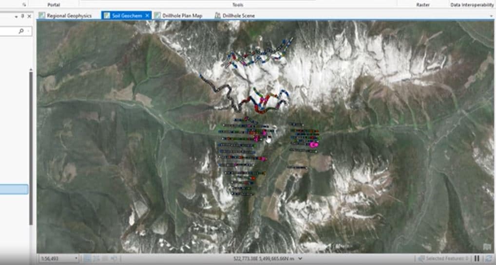
[00:02:36.340]Here, we have a satellite image

[00:02:38.040]of the project region,

[00:02:39.280]which is a rugged terrain.

[00:02:41.550]The project area is highlighted in the Southwest.

[00:02:45.000]We have regional geophysics, magnetics

[00:02:47.310]and radiometrics as gridded data.

[00:02:52.164]And we can display those grids

[00:02:53.410]using the import Geosoft Grids tool.

[00:02:59.500]Here, I’m displaying the RTP magnetics,

[00:03:02.860]and we can enhance this data

[00:03:04.380]using the Raster Appearance options.

[00:03:08.120]There are several tools here.

[00:03:09.170]I’ll just touch on a few of them briefly.

[00:03:11.590]It’s the Equalized Histogram

[00:03:13.240]and Log-Linear Classified tools.

[00:03:16.190]And these are useful for quickly applying

[00:03:18.470]a predefined colorful methods for your grids.

[00:03:22.740]The Equalized Histogram is commonly used

[00:03:25.340]with geophysical data,

[00:03:27.000]and the Log-Linear is commonly used

[00:03:28.830]with geochemical data.

[00:03:31.580]You can also import the Default Geosoft Colors

[00:03:34.190]into your project and display those as well.

[00:03:38.000]And I’m now going to talk more

[00:03:40.020]about the Quick Hillshade option.

[00:03:43.800]So the Quick Hillshade will create

[00:03:45.730]a color shaded relief image

[00:03:47.740]and display it over the top of your original data.

[00:03:51.140]And if you compare that

[00:03:52.490]with the simple color filled image

[00:03:55.570]where you have a lot of pink blobs everywhere,

[00:03:58.630]the hillshade just brings out way more detail

[00:04:02.330]for you to interpret.

[00:04:04.710]The Quick Hillshade uses the multi-directional method

[00:04:08.290]for the hillshade.

[00:04:09.700]And what that means is it takes the sun illumination angle

[00:04:12.970]from six different directions,

[00:04:15.350]and combines them into a single image.

[00:04:18.220]And what that does is it highlights relief

[00:04:21.750]in areas with high gradients or high rates of change,

[00:04:26.110]but also highlights areas

[00:04:28.050]that are relatively uninteresting or flat as well.

[00:04:35.285]What you can also do is play

[00:04:37.110]with the Traditional Hillshade options.

[00:04:40.780]And we’ll have a look at some examples of those as well.

[00:04:43.830]If you head off to the Analysis ribbon,

[00:04:45.600]and then Raster Functions,

[00:04:51.800]this will take you to here.

[00:04:53.000]And if you scroll down to the Surface tools,

[00:04:56.310]you can click on Hillshade.

[00:05:00.200]Just going to select the input grid,

[00:05:03.810]and for the Hillshade type,

[00:05:05.750]we’re going to choose Traditional this time.

[00:05:08.670]And what this allows you to do

[00:05:09.950]is choose a single Azimuth direction

[00:05:12.890]for the sun illumination,

[00:05:14.560]as well as a altitude above the horizon.

[00:05:19.730]And so I’ll show you some examples.

[00:05:26.820]So here we’re using a solar Azimuth of 315 degrees

[00:05:31.120]and 45 degrees above the horizon.

[00:05:35.820]And so, what we’re doing is taking a flashlight

[00:05:38.640]and shining on our map from the Northwest.

[00:05:41.950]And what this will do

[00:05:42.990]is preferentially highlight features

[00:05:45.600]that are running perpendicular to the Azimuth.

[00:05:50.300]So any features that are dipping towards the Northwest

[00:05:54.760]will be illuminated,

[00:05:56.280]and any features that are dipping

[00:05:58.210]away from the Northwest side

[00:05:59.630]to the Southeast will be shaded.

[00:06:04.120]And this is a useful way

[00:06:05.500]for highlighting prominent regional trends,

[00:06:09.040]cross trends, and pulling out subtle features.

[00:06:15.480]So there’s no single correct angle to use

[00:06:19.530]for your sun illumination.

[00:06:21.143]What you can do is you can try out

[00:06:23.610]a bunch of different angles,

[00:06:25.080]and this will depend on the interpreter,

[00:06:27.880]what looks good to your eye and the dataset as well.

[00:06:34.180]So, here’s an example

[00:06:36.720]of a sun illumination Azimuth of 270 degrees,

[00:06:41.140]i.e from the West.

[00:06:43.410]And, what you might notice is,

[00:06:47.560]it’s preferentially highlighting

[00:06:49.390]some of these features in the central portion

[00:06:53.010]of the survey area,

[00:06:55.120]the ones that are running North South.

[00:07:02.600]Here’s an example

[00:07:04.390]where we are using a solar Azimuth of 225 degrees.

[00:07:10.150]And what it should do is highlight

[00:07:12.740]some of these features in the Southern portion

[00:07:16.460]of the survey area,

[00:07:18.070]the ones that are running

[00:07:20.104]in this strike direction.

[00:07:32.030]We also have the first vertical derivative of the RTP.

[00:07:41.920]And this is a very popular product

[00:07:45.720]for regional studies and mapping lineaments.

[00:07:51.080]You can see that it really brings out

[00:07:52.470]the structural complexity contained within the image.

[00:07:57.560]Now, in theory, the zero contour of the 1VD,

[00:08:02.650]sits over the edge of the geologic source.

[00:08:06.200]And so what we can do,

[00:08:07.330]is we can plot the zero contour of that 1VD

[00:08:10.990]on our map as well.

[00:08:12.960]And so, we head off to the Analysis ribbon again,

[00:08:16.700]and then Raster Functions.

[00:08:20.960]This time, we’re going to browse again to the Surface tools

[00:08:26.070]and then choose contour.

[00:08:29.460]We can choose our 1VD

[00:08:33.360]and for a single contour,

[00:08:35.770]we’re going to plot one for the number of contours

[00:08:40.990]and for the contour interval,

[00:08:43.010]we’re just going to plot the zero contour.

[00:08:48.410]And when we click on Create New Layer,

[00:08:50.730]this will display in the map.

[00:09:01.330]And this is a neat way

[00:09:03.120]that you can quickly map out some of these anomalies.

[00:09:14.810]We also have Radiometrics.

[00:09:19.060]So here I’m just displaying the ratio

[00:09:22.870]of thorium to potassium.

[00:09:25.770]And this is another useful tool

[00:09:27.670]for mapping regional structure and lithology.

[00:09:31.850]So we can compare this

[00:09:34.670]with the regional geology as well.

[00:09:44.263]What we can also do, if we like,

[00:09:46.430]is plot the contours of the topography

[00:09:50.170]over the top of the radiometrics.

[00:09:53.380]So again, using the contour and options.

[00:10:02.110]Just going to choose the topography rest of this time.

[00:10:07.530]For the number of contours,

[00:10:08.920]if we want to plot multiple levels,

[00:10:13.260]you entering zero here,

[00:10:15.360]and then for the contour interval,

[00:10:17.010]we’re going to put in 100 meters,

[00:10:19.620]and every 500 meters,

[00:10:22.380]we’re going to have a bolder contour

[00:10:24.690]or a thicker contour line.

[00:10:29.060]Create New Layer,

[00:10:31.210]and this will display in the map.

[00:10:41.780]So that’s it for the geophysical data integration.

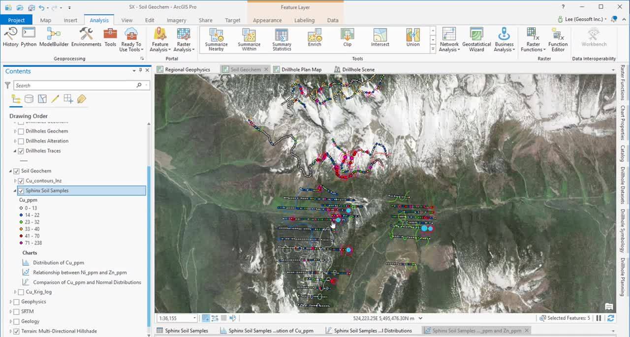
[00:10:44.740]We’re now going to zoom into our project area

[00:10:47.530]and look at some background soil samples.

[00:10:52.800]So here we have some results

[00:10:54.920]filling around a previously sampled Target area,

[00:10:58.480]as well as to analog some ridge lines.

[00:11:03.290]We can have a look at the attribute table

[00:11:05.060]for our results.

[00:11:11.695]Here we can see the different geochemical elements,

[00:11:14.140]and we can quickly grab some stats

[00:11:16.210]by right clicking on any of the attribute hitters

[00:11:18.940]and select any stats.

[00:11:22.590]This will automatically create a histogram plot.

[00:11:26.020]And we can view the chart properties

[00:11:28.530]and have a look at some basic stats.

[00:11:33.860]I’m just going to turn on the mean and standard deviation,

[00:11:37.900]in our chart over here.

[00:11:44.610]And so this can be useful

[00:11:46.300]for helping you to classify your data,

[00:11:49.580]and help set up your graduated symbols.

[00:11:55.430]We’re also interested in dependent

[00:11:57.470]or correlated attributes.

[00:11:59.290]And there are a number of different charts

[00:12:01.060]that you can use to plot your data.

[00:12:08.900]So we can go to Create Chart,

[00:12:11.420]and we’re going to have a look at the QQ Plot.

[00:12:16.430]The QQ Plot plots our data distribution

[00:12:19.690]against a normal distribution.

[00:12:21.860]You can also compare it

[00:12:22.870]against some other transformations as well.

[00:12:27.670]There’s the log transform and also the square root.

[00:12:31.740]Which is similar to the log transform,

[00:12:33.400]except it allows us

[00:12:34.570]to include negative and zero values as well,

[00:12:37.940]which the log transform cannot.

[00:12:42.050]Here, we can see

[00:12:42.883]that the copper has a log normal distribution.

[00:12:45.910]Selecting the top copper results,

[00:12:53.000]we’ll automatically highlight these samples

[00:12:56.370]in the attribute table,

[00:12:57.580]as well as display them and highlight them in the map.

[00:13:01.640]We can also compare these selective results

[00:13:03.690]with a scatter plot of nickel versus zinc.

[00:13:07.800]And here we can see

[00:13:08.670]those selected anomalous copper results.

[00:13:12.750]Again, if you have gridded data,

[00:13:16.250]you can import that into the project as well.

[00:13:19.000]And so here, I’ve got a grid of the copper results,

[00:13:23.850]which was created using the creaking algorithm

[00:13:27.550]in log transform.

[00:13:35.260]As well, we can plot the contours

[00:13:38.030]for that Raster as well.

[00:13:47.610]Next, I’m going to display the colors

[00:13:49.190]around a known soil anomaly.

[00:13:57.130]The drilling results include color survey

[00:14:00.280]and down hole data.

[00:14:01.650]These are imported into a file Geodatabase,

[00:14:04.810]and stored as a drillhole feature dataset.

[00:14:15.470]Here’s a plan view of the drillholes

[00:14:17.070]with the traces projected to the surface.

[00:14:21.800]There are several options now

[00:14:23.120]for adding drillhole data to the map.

[00:14:25.460]The first way is using the catalog.

[00:14:28.290]And here you can drag and drop features

[00:14:30.410]directly into the map.

[00:14:33.030]The thing with dragging and dropping from here though,

[00:14:35.010]is that the symbology is going to inherit

[00:14:38.000]single colored symbols only.

[00:14:40.250]And so you’re going to have to spend at least some time

[00:14:42.070]setting up the symbology

[00:14:43.270]in order to analyze your data.

[00:14:46.570]You can also add drillhole data to the map

[00:14:48.470]using the Target ribbon,

[00:14:50.630]Add to Map, Drillhole Data.

[00:14:56.500]Here we have two tabs.

[00:14:59.240]The Datasets tab is a cleaner view of the catalog

[00:15:05.520]and it groups some of the related features.

[00:15:10.780]You can drill down into the different attribute tables

[00:15:14.460]and see the data contained within them.

[00:15:17.520]And if you drag and drop from here,

[00:15:23.480]you’ll notice that it will display

[00:15:24.790]with some default predefined symbology.

[00:15:29.391]And so that you can immediately start to see

[00:15:31.000]some variation within your drillholes.

[00:15:41.450]The drag and drop feature from the Datasets tab

[00:15:44.580]is one layer at a time.

[00:15:48.110]If you want to quickly add multiple layers,

[00:15:51.000]you can use the Add Data tab.

[00:15:52.840]And here we have some switches

[00:15:54.760]that you can just go through

[00:15:56.780]and select as many as you like.

[00:16:01.860]And when you hit Apply,

[00:16:05.050]these will all be displayed in the map

[00:16:06.870]using some predefined symbology for you.

[00:16:11.210]I’m just going to turn on some layers

[00:16:12.810]that I’ve already gotten here.

[00:16:16.130]So here we’ve got the copper results.

[00:16:18.450]If you don’t like the predefined symbology

[00:16:20.920]that we’ve created for you already,

[00:16:23.420]you can always right click and use the pro tools

[00:16:26.150]to further modify the symbology.

[00:16:32.600]Another way that you can modify the symbology

[00:16:35.780]is to use the Target ribbon symbology,

[00:16:39.630]and then this drillhole Symbology option.

[00:16:49.160]And here we’ve taken some

[00:16:50.880]of the frequently used symbology options.

[00:16:53.940]For example, color and size by values.

[00:16:57.880]And we’ve put it all into one place for you.

[00:16:59.680]So here we can set the color field

[00:17:02.190]using the Moli values.

[00:17:03.980]The size will also be based on the assay values,

[00:17:10.670]and we can have a graduated symbol size

[00:17:14.230]and see what that looks like.

[00:17:21.620]We can make that a little bit bigger.

[00:17:34.250]And so here,

[00:17:35.083]we’ve got more of a traditional histogram plot

[00:17:38.730]that you might be used to seeing.

[00:17:46.600]We can also display our rock types

[00:17:52.080]and offset them from the drillhole trace as well,

[00:17:54.350]so that we can see some correlation there as well.

[00:18:05.530]Once you’ve got the symbology looking just right,

[00:18:08.010]a good idea is to start to save your symbologies

[00:18:11.270]as you work through.

[00:18:13.100]And you can do this by right clicking

[00:18:14.270]on any of the layers and going to Drillhole Symbology,

[00:18:17.480]and then Save and Set as Default.

[00:18:21.120]Clicking on this will open up the drillhole Symbology

[00:18:27.600]and take you to the Manage tab.

[00:18:32.420]And here we can see those saved symbologies.

[00:18:38.540]You can also head off to this Set Defaults tab,

[00:18:42.200]and you can assign those templates

[00:18:45.640]for your different layers.

[00:18:51.410]And so, any time you add these layers to the map,

[00:18:55.280]whether it’s a 2D map or 3D scene,

[00:18:57.840]that layer is going to inherit your saved template

[00:19:00.380]for the symbology.

[00:19:03.370]Well, that being said,

[00:19:04.270]we’re going to now jump into a 3D drillhole scene.

[00:19:12.380]And the new drillhole scene option

[00:19:14.270]is going to create a new local scene

[00:19:16.790]and automatically load in your drillholes

[00:19:20.110]and hole traces.

[00:19:23.860]If you have any base maps or world imagery

[00:19:26.730]turned on in the scene,

[00:19:28.540]you’ll probably find that by default,

[00:19:30.160]that’s going to extend out to the edge of the horizon.

[00:19:32.500]And this can make it quite challenging

[00:19:34.530]to navigate around the 3D scene

[00:19:36.180]and get the right zoom level.

[00:19:38.950]What you can do in this case

[00:19:40.050]is clip the scene to the extents of your drillholes.

[00:19:46.560]We also have some predefined viewing angles

[00:19:49.080]to help you as well.

[00:19:54.330]And I’m just going to zoom this in,

[00:19:57.090]so that we can see the data.

[00:20:00.350]And here we’ve got the assays loaded in the game

[00:20:03.720]and they’ve been colored and sized by their values.

[00:20:07.690]But what I’d like to do now

[00:20:08.810]is incorporate some models of this data.

[00:20:13.650]And there are a couple of ways

[00:20:15.130]that we can incorporate the information

[00:20:17.730]from 3D voxel models.

[00:20:20.780]The S3 filed Geodatabases don’t yet have

[00:20:24.100]a feature class that can store 3D voxels.

[00:20:27.570]But what we can do is we can import slices

[00:20:31.500]that have been extracted from the voxel instead.

[00:20:34.960]So we can import those using the Geosoft Grids option.

[00:20:37.680]And let me just turn on two of those grids

[00:20:41.940]that have been extracted

[00:20:42.810]from a 3D grid of the assays.

[00:20:52.280]Here they are.

[00:20:55.710]Just look at it from another angle.

[00:21:03.440]And so here are those gridded section values of the assays.

[00:21:18.050]We can also bring in 3D models

[00:21:21.300]of the data as well.

[00:21:23.020]And so here, I’ve also got … let’s turn on …

[00:21:28.630]some isosurfaces,

[00:21:30.040]which have been extracted from the same voxel,

[00:21:32.190]or gray shells, if you will.

[00:21:37.290]These were imported

[00:21:39.010]using the import Subsurface Mesh tool.

[00:21:43.770]And these ones came from a Geosurface file.

[00:21:49.080]We can also import models of the geology.

[00:21:54.500]So I’m going to turn on my 3D model

[00:22:02.220]of the lithology,

[00:22:03.053]which has been created in this case

[00:22:04.990]through Y framing, in Geosoft Target.

[00:22:17.760]You can also import 3D models

[00:22:20.740]and meshes from OMF files.

[00:22:23.320]And OMF files are supported by Geosoft and Leapfrog.

[00:22:27.790]So if you have modeled up any surfaces

[00:22:29.690]in Leapfrog, you’re going to export them to an OMF file

[00:22:31.890]and display them in your 3D scenes,

[00:22:34.556]Micromine Deswik also support OMF files

[00:22:37.250]as well as few others, I think.

[00:22:44.040]What we’re going to do now

[00:22:44.910]is slice some sections out of our 3D scene.

[00:22:48.450]So I’m going to swing us around back to the top.

[00:22:58.430]Creating sections is done in the 3D scene

[00:23:00.830]by going to the Subsurface tools

[00:23:02.560]and clicking on Section.

[00:23:06.720]Here, it brings up the Section tool.

[00:23:08.430]We can click on Create New Section.

[00:23:15.040]And I’ll just turn off the elevation surface

[00:23:18.540]so that we can see our drillhole traces.

[00:23:22.000]Zoom in a bit.

[00:23:25.140]It’s also a bit easier to digitize your Section window

[00:23:28.720]by changing the drawing angle to parallel.

[00:23:33.710]And that just helps you line up your section

[00:23:35.440]and see what objects actually fall

[00:23:38.090]within that Section window.

[00:23:41.920]So we can now start digitizing

[00:23:44.380]the front face of the section.

[00:23:51.120]And we can drag out the thickness

[00:23:55.580]and then lock in the extents.

[00:23:58.320]Once we’ve locked in the extents,

[00:24:00.780]information about the center point of the section,

[00:24:04.650]the orientation and extents of the section,

[00:24:07.770]can then be modified explicitly over here.

[00:24:10.890]You can click on any of these values

[00:24:12.560]and use the slider to increase or decrease

[00:24:16.040]any of those values.

[00:24:17.010]You can also just type in

[00:24:19.590]the values that you want as well.

[00:24:28.372]What you can also do

[00:24:29.205]is clip the section to the extents.

[00:24:36.240]And we can have a look at it

[00:24:38.900]from the front as well.

[00:24:41.960]And here I might want to increase the vertical extents

[00:24:48.860]and maybe the length as well.

[00:25:08.300]If you’d like to create multiple sessions,

[00:25:10.480]or batch create some sections,

[00:25:12.100]you can use the create Off Sections option over here.

[00:25:15.970]If you turn this on,

[00:25:18.250]you can select the number of sections

[00:25:20.130]that you’d like to create,

[00:25:22.690]and the offset between each section.

[00:25:31.440]If you’d like these sections to go in the other direction,

[00:25:35.480]you can just put a minus sign

[00:25:38.090]in front of the separation here,

[00:25:41.890]and that will change it to go the other way.

[00:25:54.170]Once you’re happy with the way the section looks,

[00:25:56.590]you can click on Save.

[00:25:58.950]And before you do that,

[00:25:59.783]you can actually also change

[00:26:00.780]the name of the section.

[00:26:01.720]That’s going to be stored as well.

[00:26:04.240]Clicking on Save will then take you

[00:26:05.640]to the Manage Sections tab over here.

[00:26:13.330]Here we can turn on which sections we’d like to use.

[00:26:19.190]We can sort these sections

[00:26:22.200]by direction, say from North to South.

[00:26:27.700]And if at any time we want to modify

[00:26:30.470]any of these saved sections,

[00:26:32.240]we can head off to the Modify tab,

[00:26:35.710]select the section that we want to work with,

[00:26:39.210]and then just modify any of the features

[00:26:43.520]of that section down here.

[00:26:49.820]Once we’ve created our sections

[00:26:51.610]and we just want to get a quick view

[00:26:55.040]of any of the sections

[00:26:56.100]that we’ve created and saved,

[00:26:58.030]we can use the Section View tool over here.

[00:27:03.000]So the Section View will bring up the first section

[00:27:06.210]that you’ve created.

[00:27:07.390]And you can use the dropdown

[00:27:09.920]and select different sections,

[00:27:11.240]or you can use these cursor down and cursor up buttons

[00:27:16.100]to cycle through your saved sections.

[00:27:22.920]We can turn on different layers.

[00:27:32.000]We can further clip the section

[00:27:35.730]to the center slice of it.

[00:27:43.150]We can draw on pierce points with drillholes

[00:27:47.220]and the center slice,

[00:27:52.090]as well as pierce points with the front and the back

[00:27:55.810]of the Section window as well.

[00:28:00.140]If I just spin this section to the left side,

[00:28:06.300]you can see those center pierce points,

[00:28:09.850]as well as the front and back pierce points as well.

[00:28:20.900]You can have a look at the section from the top.

[00:28:26.580]You can also drape any geo-reference images

[00:28:32.390]onto your elevation surfaces

[00:28:34.700]so here we’ve got a map of the alteration

[00:28:39.850]as a GeoTIFF.

[00:28:48.810]And next we’re actually going to use our Section view

[00:28:51.760]to plan some new proposed drillholes.

[00:28:56.740]So the drillhole planning tool

[00:28:58.040]is a new feature in version 2.1

[00:29:01.010]of Target Practice Pro,

[00:29:03.480]which will be getting released soon.

[00:29:05.900]And we’ll have a look

[00:29:06.733]at this drillhole planning tool now.

[00:29:10.300]I’m going to close some of these windows here

[00:29:13.790]to give us some bit more screen real estate.

[00:29:18.720]And I’m going to split my views

[00:29:21.470]between the drillhole scene and the 2D plan view.

[00:29:30.000]Zoom in a bit.

[00:29:32.360]We can select the section

[00:29:34.040]that we’d like to digitize from.

[00:29:38.620]And there are a couple of ways

[00:29:39.530]you can plan a new home

[00:29:41.160]and we’ll speak about the first one.

[00:29:42.840]Using a color location and a Target location

[00:29:45.420]to calculate the drillhole trace.

[00:29:48.370]So we can click on the color location

[00:29:50.490]and pick a spot where we want the color

[00:29:54.000]and that location will update

[00:29:55.950]in the plan view as well.

[00:29:59.030]We can get our elevation value for the color

[00:30:01.920]from a topography raster.

[00:30:04.810]Just browse and select my DTM surface.

[00:30:11.520]And you’ll see the Z value will update accordingly.

[00:30:17.100]We can pick a Target location

[00:30:24.470]and the whole length Azimuth

[00:30:26.850]and depth of the hole be automatically calculated

[00:30:29.570]and also displayed in the 2D plan view as well.

[00:30:36.280]If we’d like we can use a color

[00:30:38.690]and then hole trace information

[00:30:40.680]to calculate the Target location instead.

[00:30:44.510]So let’s say for the hole length,

[00:30:46.970]maybe, we only want it to be

[00:30:52.660]600 meters,

[00:30:55.710]and we can see that getting updated in the map.

[00:30:59.570]Similarly, if we want say our inclination,

[00:31:03.290]instead of minus 71,

[00:31:05.210]we actually wanted it to be minus 60,

[00:31:12.900]and this will calculate a new Target location for us.

[00:31:20.700]We can give it a new name,

[00:31:29.300]and a description.

[00:31:33.990]And when we save this,

[00:31:35.050]it’ll create a new feature class

[00:31:37.720]for our planned drillholes

[00:31:38.830]and save it in our file Geodatabase.

[00:31:44.700]To finish things off,

[00:31:45.580]we’re just going to touch on some tools

[00:31:47.400]for allowing you to share your projects

[00:31:50.460]and collaborate with others.

[00:31:53.730]And we’re going to head off to the Share ribbon.

[00:31:57.560]And so there are a couple of ways you can do this.

[00:31:59.680]One is to package up your entire project

[00:32:03.630]and this will package it up into a single file,

[00:32:05.990]which you can email or share with your colleagues,

[00:32:09.810]however you like.

[00:32:11.810]Another neat way is to use these Web Scenes.

[00:32:15.960]And you can create a web scene for your 3D scenes.

[00:32:21.620]And what this will do is it’ll create a web link,

[00:32:25.520]that you can open up and your web browser,

[00:32:29.710]email to colleagues.

[00:32:30.830]They can also view it

[00:32:32.350]in their smart devices or tablets.

[00:32:36.670]And what this gives you is a 3D scene viewer,

[00:32:39.770]which you can interact with.

[00:32:43.620]You can spin it around.

[00:32:52.490]Let me just rotate it around here.

[00:32:54.860]You can also turn on and off different layers

[00:32:57.040]and view other data that’s already stored within there.

[00:33:09.560]This is quite a handy tool

[00:33:11.390]for taking your projects out of the office

[00:33:14.120]and on the go with you as well.

[00:33:24.250]That being said,

[00:33:25.260]I’m going to jump back to my PowerPoint.

[00:33:39.120]The next Technical Tuesday session is on June 30th

[00:33:42.800]and the title is

[00:33:43.633]“Branch out Your collaboration with Central.”

[00:33:46.690]You can sign up for any of our online events

[00:33:48.660]through sequent.com/events.

[00:33:53.630]And if you’d like to ask any follow-up questions,

[00:33:56.160]or if you need help with anything

[00:33:58.080]in Target Practice Pro or otherwise,

[00:34:00.900]you can contact our global support team

[00:34:03.390]through [email protected].

[00:34:06.590]Thanks for watching.