Technical Tuesdays: Advanced surface editing in Leapfrog Geo

During this technical workshop, we discuss advanced surface editing tips. Learn how to create accurate domains by developing a deeper understanding of intrusion parameters and the ways surfaces can be edited.

 

Overview

Video Transcript

[00:00:00.595]
(upbeat music)

[00:00:04.520]
<v Ivan>Welcome to the technical</v>

[00:00:05.590]
Tuesdays webinars series.

[00:00:07.060]
My name is Ivan Naumenko

[00:00:08.350]
and I’m a Project Geologist with Seequent Australia.

[00:00:11.050]
Today’s webinar topic is advanced surface editing,

[00:00:13.940]
and we will focus on the intrusion surface type.

[00:00:19.690]
The Seequent solution encompasses

[00:00:20.870]
a range of software products applicable for use

[00:00:23.040]
across the money and value chain.

[00:00:24.980]
Today I’ll focus on Leapfrog Geo.

[00:00:27.100]
If you would like to find out more about other solutions,

[00:00:29.460]
please contact our support and sales stuff.

[00:00:33.710]
Today, I’ll focus on advanced surface editing techniques,

[00:00:36.450]
tips and tricks when using intrusion surface type.

[00:00:39.200]
We will we dig deeper into the settings menu

[00:00:41.210]
and we’ll review surface settings,

[00:00:43.580]
which you can adjust to achieve better results

[00:00:46.370]
when trying to make an intrusion surface to fit your data.

[00:00:50.090]
Also, we will discuss a couple of scenarios

[00:00:52.030]
that people are commonly facing

[00:00:53.300]
when modeling in Leapfrog Geo.

[00:00:56.408]
I will briefly go over the concept of intrusion surface type

[00:00:59.020]
and its main applications.

[00:01:01.280]
I will review the structure of intrusion surface,

[00:01:03.400]
In other words, how it’s generated and what it is based on.

[00:01:07.170]
We will look at trends editing the intrusion surface

[00:01:09.820]
by applying trends, linear or structural.

[00:01:12.470]
We will look at the intrusion values composite

[00:01:14.390]
in generation settings for intrusion surfaces

[00:01:16.690]
and see how these settings

[00:01:17.690]
can affect the result in surface.

[00:01:20.690]
Advanced surface settings, additional settings

[00:01:23.357]
that are available for intrusion surfaces and what they do.

[00:01:26.690]
Also we’ll have a brief look at the guide points.

[00:01:30.170]
What are those and how you can use guide points

[00:01:32.250]
to adjust your intrusion surface?

[00:01:35.210]
Before I jumped to the live demo

[00:01:36.430]
for the benefit of those who are new to LeapFrog Geo,

[00:01:38.680]
I would like to explain what the intrusion surface is.

[00:01:41.450]
Intrusion contact surfaces are rounder in shape

[00:01:43.560]
with an interior lithology that represents

[00:01:45.530]
the intrusion of lithology.

[00:01:47.200]
The intrusion removes existing lithologies and replaces them

[00:01:49.980]
with the intrusive lithology

[00:01:51.340]
on the youngest side of the contact surface.

[00:01:53.890]
Often the older side of the intrusion contact surface

[00:01:56.610]
is labeled as unknown, as typically intrusions displaced

[00:02:00.120]
multiple older lithologies.

[00:02:01.970]
Intrusion surfaces can be made from a range

[00:02:04.020]
of juicing different data types,

[00:02:05.530]
such as drilling polar lines,

[00:02:08.100]
GIS structural disks and points.

[00:02:11.740]
Now I’m going to switch to Leapfrog Geo

[00:02:13.460]
and continue with a live demo.

[00:02:17.150]
During this session,

[00:02:17.983]
we will focus on using the intrusion surfaces

[00:02:19.950]
in the construction of Geological Models.

[00:02:22.180]
Please keep in mind that intrusion surfaces

[00:02:23.970]
can be used to model porphyries, pegmatites or shells,

[00:02:27.100]
contamination in internal waste pockets,

[00:02:29.230]
as well as any other type of contact,

[00:02:31.070]
which generally requires a specific category of intervals

[00:02:34.650]
to be in close by contact and surface.

[00:02:37.550]
I have saved a couple of things to speed up the process

[00:02:39.660]
of switching between the views during this demo.

[00:02:42.040]
So let me quickly switch to the next scene.

[00:02:45.240]
First, let me start with an overview of the project.

[00:02:47.920]
This is a train in porphyry copper gold project

[00:02:49.950]
which has a number of drill holes intersecting

[00:02:51.680]
the various lithological units and a topographical surface

[00:02:54.490]
with some jazz data draped on it.

[00:02:57.270]
The units include a quartz vein, dollar ride dikes,

[00:03:00.310]
overburden unit, volcanic sediments,

[00:03:02.400]
granite diorite and quartz porphyry units.

[00:03:04.900]
The main focus of today’s session will be

[00:03:06.610]
on the last two units,

[00:03:07.720]
the granite diorite and the quartz porphyry.

[00:03:10.300]
For the benefit of those who are new

[00:03:11.570]
to Leapfrog Geo software,

[00:03:12.760]
I’ll briefly go through the process

[00:03:14.160]
of creating an intrusion surface.

[00:03:16.440]
I have already created a geological model

[00:03:18.120]
in which I am going to generate an intrusion surface.

[00:03:21.210]
Right click on the surface chronology object

[00:03:23.000]
in geological model.

[00:03:24.610]
Select the intrusion option

[00:03:25.810]
from the list of available objects.

[00:03:28.190]
If you would like to use your drill hole data

[00:03:29.850]
to create an intrusion surface,

[00:03:31.310]
then select new intrusion from basic lithology.

[00:03:35.090]
The first thing we need to do here,

[00:03:36.470]
is select the primary lith unit.

[00:03:38.240]
I will be building quartz porphyry intrusion,

[00:03:40.080]
so I will select quartz porphyry as a primary unit.

[00:03:44.180]
The next step is selecting the exterior and ignored units.

[00:03:47.690]
The contact in older lithologies

[00:03:49.830]
will stay under the exterior lithologies

[00:03:51.570]
and all younger ones will go into the ignored column.

[00:03:55.040]
As you can see, I have generated an intrusion surface

[00:03:57.480]
around quartz porphyry drill hole into walls.

[00:04:00.200]
If I have a closer look,

[00:04:01.460]
I can see that quartz porphyry contacts with the vein

[00:04:03.950]
and dike intervals have been ignored.

[00:04:06.850]
This is because I have set those lith units as younger.

[00:04:10.890]
Let’s have a closer look at the geological model

[00:04:12.850]
I have generated earlier.

[00:04:14.370]
As you can see, we have a sequence

[00:04:16.030]
of volcanic sediments model as a country rock unit.

[00:04:19.020]
We also have two intrusions,

[00:04:20.750]
the granite diorite and the porphyry,

[00:04:23.130]
all of these are caught by younger veins and dikes,

[00:04:25.400]
then clicked by the overburden unit at the top.

[00:04:28.550]
This surfaces have not been modified in any way

[00:04:30.710]
and are based purely on the drill hole data.

[00:04:33.880]
You might have already noticed a couple of issues

[00:04:35.680]
with the surfaces that need to be addressed.

[00:04:38.920]
Upon closer inspection we can see that,

[00:04:40.640]
there are problems with quartz porphyry intrusion surface.

[00:04:43.070]
Right in the center, there is a big gap split

[00:04:44.850]
in the quartz porphyry surface into parts,

[00:04:47.270]
as well as the small part of the surface disconnected

[00:04:49.810]
from the main body in depth.

[00:04:52.860]
These problems are likely to be caused by past drilling data

[00:04:55.900]
prompted to close off the intrusion surface rather

[00:04:58.340]
than generating a container surface.

[00:05:01.050]
Take into account a quite simple shape

[00:05:02.830]
of this porphyry intrusion.

[00:05:03.880]
my suggestion would be to avoid manual explicit edits

[00:05:06.660]
until we have tested different intrusion settings

[00:05:08.920]
to make the surface fit the data.

[00:05:11.830]
You will notice how the intrusion appears rounder,

[00:05:14.080]
as algorithm searches equally in all directions

[00:05:16.390]
to find correspondent intercepts.

[00:05:18.550]
My first thought would be to try using a linear trend

[00:05:21.090]
and see if applying direction of greatest continuity

[00:05:23.720]
will help to fix this problem.

[00:05:26.220]
To set the trend,

[00:05:27.053]
I’ll be using the tool called moving plane.

[00:05:29.080]
I will position the model in the scene so I can draw a plane

[00:05:32.030]
along this strike of the porphyry.

[00:05:34.000]
Please note that the moving plane doesn’t have to go

[00:05:36.040]
precisely through the center of the porphyry intrusion.

[00:05:38.690]
I will only use the plane to copy deep inasm values

[00:05:41.610]
to the intrusion surface.

[00:05:43.660]
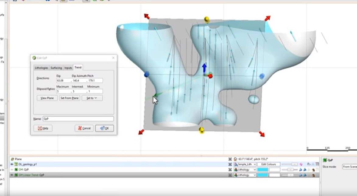
Now I’m ready to apply the trend value

[00:05:45.720]
to my quartz porphyry intrusion surface.

[00:05:48.170]
Double click on the quartz porphyry intrusion,

[00:05:49.790]
and navigate to the trend tab in dialog window.

[00:05:53.510]
You can see that there is a set from plane button,

[00:05:55.550]
which allows you to copy the deep

[00:05:56.940]
as in with impeach information from the moving plane

[00:05:59.210]
to the intrusion surface.

[00:06:01.430]
The set to button allows you to copy the trend values

[00:06:04.130]
from other objects in your project,

[00:06:06.860]
or reset the trend back to isotropic.

[00:06:09.580]
You can control the strength of the trend

[00:06:11.180]
by adjusting the ellipsoid ratio values.

[00:06:14.700]
The ellipsoid ratio is determined that relative shape

[00:06:17.050]
and strength of the ellipsoids in the scene.

[00:06:21.220]
The maximum value is the relative strength in the direction

[00:06:23.930]
of the green line on the moving plane.

[00:06:25.960]
You can adjust it by left-clicking,

[00:06:27.650]
and activating controls on the moving plane.

[00:06:30.240]
The intermediate value is the relative strength

[00:06:32.300]
in the direction perpendicular to the green line

[00:06:34.300]
on the moving plane.

[00:06:35.970]
The minimum value is a relative strength

[00:06:37.960]
in the direction orthogonal to the plane.

[00:06:40.610]
As drilling is most often perpendicular to the orbital,

[00:06:43.380]
in the majority of cases, your minimum values,

[00:06:45.360]
should be your lowest number.

[00:06:48.040]
With the ellipsoid ratios, what is important,

[00:06:50.010]
is the ratio of the numbers you enter.

[00:06:51.900]
The higher the maximum and the intermediate numbers,

[00:06:54.040]
the stronger the trend is applied in that direction.

[00:06:57.240]
Things to consider when applying trends

[00:06:58.920]
are the geometry of the orbital,

[00:07:00.430]
as well as your drill holes pacing.

[00:07:02.840]
The thinner the intercepts

[00:07:03.950]
or the wider the drill holes are apart,

[00:07:05.810]
the stronger trend you may need to apply.

[00:07:08.100]
When applying a trend,

[00:07:09.180]
you may need to try a few different combinations of numbers

[00:07:11.860]
to create the optimal shape for your deposit.

[00:07:16.120]
I will click Concept From Plane and Okay

[00:07:18.220]
to apply the changes.

[00:07:21.350]
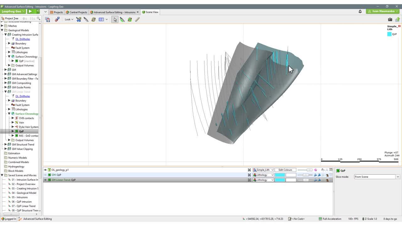
As you can see, the shape of the intrusion surface

[00:07:23.190]
has changed significantly,

[00:07:24.570]
and now it fits the data quite well.

[00:07:27.630]
Linear trends work very well on relatively simple deposits,

[00:07:30.520]
but quite often the structure and shape of the deposit

[00:07:32.990]
are much more complex and follow non-linear trends.

[00:07:36.690]
Leapfrog Geo has a tool called structural trend.

[00:07:39.100]
It allows you to apply a nonlinear trend

[00:07:41.240]
to an intrusion surface.

[00:07:43.080]
Structural trends create a flat ellipsoid anisotropy

[00:07:45.690]
that varies in direction with its inputs.

[00:07:48.600]
To create a new structural trend,

[00:07:50.010]
right click on the Structural Trends folder,

[00:07:51.990]
in the structural modelling folder

[00:07:53.930]
and select New Structural Trend.

[00:07:56.910]
The structural trend window will appear.

[00:08:00.110]
Structural trends can be created from surfaces

[00:08:02.210]
and from structural data.

[00:08:04.460]
Click add to select from the suitable inputs

[00:08:06.420]
available in the project.

[00:08:07.920]
I have generated a mash by creating a series of polar lines

[00:08:10.860]
representing the trend orientation and given locations.

[00:08:13.990]
And now I will use this mesh

[00:08:15.550]
as an input for my structural trend.

[00:08:18.630]
I won’t spend too much time explaining all settings

[00:08:20.890]
available for structural trends.

[00:08:22.810]
You can find more information about structural trends

[00:08:24.930]
in the help files or by contacting Leapfrog support team

[00:08:27.510]
in your region.

[00:08:29.890]
Now that I have my structural trend object ready,

[00:08:32.150]
I have to change some settings

[00:08:33.270]
in my quartz porphyry intrusion before I can apply

[00:08:35.755]
this structural trend to it.

[00:08:37.849]
I will double-click on the quartz porphyry intrusion object

[00:08:39.880]
to open the settings window,

[00:08:41.590]
then navigate to the surface in tab

[00:08:43.385]
and click on the additional options.

[00:08:44.790]
Then navigate to the interpolate tab,

[00:08:47.418]
I have to switch to the interpolate tab

[00:08:48.620]
from linear to spheroidal

[00:08:49.660]
before I can apply my structural trend.

[00:08:51.840]
You can read more about the interpolate settings

[00:08:53.850]
for intrusion surfaces in help files.

[00:08:57.120]
Now I can move back to the trend tab

[00:08:58.800]
and select the structural trend

[00:08:59.940]
that I would like to apply to this intrusion.

[00:09:02.710]
The outside value is a long range main value of the data,

[00:09:06.170]
such a new value of negative one for intrusions,

[00:09:08.500]
where the positive valleys are on the inside

[00:09:11.500]
and positive one for other surfaces

[00:09:13.860]
will result in a smoother surface in most cases.

[00:09:17.110]
Now we can see how the quartz porphyry intrusion

[00:09:19.250]
is following the structural trend.

[00:09:21.180]
We can compare it to the core support for intrusion surface,

[00:09:23.950]
with a linear trend applied to it.

[00:09:45.250]
Let’s dig a little bit deeper

[00:09:46.500]
and see how Leapfrog generates intrusion surfaces.

[00:09:49.580]
Leapfrog starts by extracting the intrusion intervals

[00:09:51.610]
from the drill hole database

[00:09:52.840]
and converting them into intrusion points.

[00:09:55.620]
Leapfrog converts the categoric interval data

[00:09:57.750]
into numeric point data.

[00:10:00.430]
We’ll now look closer at the point generation parameters.

[00:10:03.463]
I will double-click on the intrusion points,

[00:10:06.410]
the edit intrusion window will appear

[00:10:08.520]
displaying the point generation tap.

[00:10:10.530]
Here the surface and volume points are displayed

[00:10:12.550]
to show the effects of the surface offset distance

[00:10:15.180]
and background field space and parameters.

[00:10:18.040]
The surface offset distance parameters,

[00:10:19.690]
sets the top and bottom ends of the interval

[00:10:22.160]
and affects how surface behaves

[00:10:23.860]
when it approaches a contact point.

[00:10:26.110]
The smaller distance restricts the angles that an approach

[00:10:28.910]
and surface can take.

[00:10:30.690]
Another factor that affects the angles a surface will take,

[00:10:33.310]
is whether or not trend has been applied to the surface.

[00:10:37.480]
The background field space in parameter,

[00:10:38.970]
determines the approximate length of the segments

[00:10:41.230]
in the remaining intervals.

[00:10:43.660]
If the remaining interval is not a multiple

[00:10:45.350]
of the background field space and value,

[00:10:47.210]
Leapfrog will automatically adjust the spacing

[00:10:49.700]
to an appropriate value.

[00:10:51.800]
A smaller value for background field space

[00:10:53.910]
means high resolution

[00:10:55.240]
and therefore slightly smoother surfaces.

[00:10:57.440]
However, the computation can take longer.

[00:11:01.200]
Now let’s have a look at the intrusion points

[00:11:02.790]
composite in settings.

[00:11:04.170]
This can be accessed by double clicking

[00:11:05.760]
on the intrusion points and navigating to the composite tab

[00:11:08.670]
in the dialogue window.

[00:11:11.140]
Sometimes unit boundaries are poorly defined with fragments

[00:11:13.800]
of other lithologist within the lithology of the interest.

[00:11:17.160]
This can result in very small segments

[00:11:18.750]
near the edges of the lithology of interest.

[00:11:21.200]
Modelling defined detail is not always necessary,

[00:11:23.870]
And so compositing can be used to smooth these boundaries.

[00:11:28.150]
As you can see it Leapfrog applies automatic composition

[00:11:30.350]
into the input data.

[00:11:31.910]
This setting can be manually adjusted.

[00:11:34.040]
The automatic setting values depends

[00:11:35.820]
on the resolution settings applied to the surface

[00:11:38.813]
and set to half of the resolution value.

[00:11:41.030]
In this example the surface resolution is set to 30,

[00:11:44.170]
therefore the automatic compositing values are set to 15.

[00:11:49.040]
Might have already noticed that a short segment

[00:11:50.810]
in the center of the screen has been filtered out,

[00:11:53.010]
due to the compositing settings.

[00:11:55.330]
There are a couple of ways in which you can bring it back.

[00:11:59.520]
First, adjust the surface resolution value

[00:12:01.550]
to allow for shorter segments to be included.

[00:12:03.900]
Second, untick the simplify geology

[00:12:06.140]
by filtering short segments box.

[00:12:08.350]
And the third way is to adjust the filtering values,

[00:12:10.540]
so the short intervals of specific length

[00:12:12.800]
are included in the modeling.

[00:12:15.160]
Now I’ll try to untick the box,

[00:12:16.650]
simplify geology by filtering short segments,

[00:12:19.030]
then click Okay.

[00:12:21.020]
As you can see,

[00:12:21.853]
the short segments has now been included

[00:12:23.380]
in the construction of the intrusion surface.

[00:12:26.830]
There will be situations when dealing with photo models,

[00:12:29.290]
in which you might have limited data

[00:12:30.940]
in one or more of your fault blocks.

[00:12:34.090]
In such cases,

[00:12:34.923]
you may want to switch off the boundary filter

[00:12:36.950]
to allow Leapfrog, to use data outside of the domain

[00:12:39.400]
to inform the surface.

[00:12:41.970]
You can turn the screen

[00:12:42.830]
that the quartz porphyry intrusion surface

[00:12:44.740]
in one of the fault blocks

[00:12:45.980]
is based only on a single interval

[00:12:48.570]
and very much unconstrained at depth.

[00:12:51.260]
To rectify this issue, I will try

[00:12:52.960]
and adjust the boundary filter settings.

[00:12:56.530]
You can access the boundary filter settings,

[00:12:58.260]
by double clicking on the surface

[00:12:59.750]
and navigating to the surface and tap.

[00:13:02.150]
From the dropdown menu, under the boundary filter field,

[00:13:05.020]
select one of the settings you would like

[00:13:06.510]
to apply to this particular surface.

[00:13:08.940]
The boundary often intrusion

[00:13:10.170]
can be the geologic model boundary or fault block boundary.

[00:13:14.250]
The boundary filter setting determines how data used

[00:13:16.720]
to define the surface is filtered.

[00:13:18.850]
When it’s switched off, data is not filtered.

[00:13:21.970]
When it’s set to all data, all data is filtered.

[00:13:25.560]
When it’s set to drilling only, only drill hole data

[00:13:27.900]
and data objects derived from drill hole data are filtered.

[00:13:31.490]
When it’s set to custom, only the data objects

[00:13:33.490]
specified in the inputs tab are filtered.

[00:13:37.160]
I will switch the boundary filter off now

[00:13:38.840]
and see how this affects the shape

[00:13:40.260]
of the quart porphyry intrusion surface.

[00:13:43.150]
Now that Leapfrog uses the data outside the current boundary

[00:13:46.280]
set to the surface.

[00:13:47.390]
You can see that the shape

[00:13:48.580]
of the intrusion surface has changed significantly.

[00:13:51.460]
Turning off the boundary filter can also be beneficial

[00:13:53.860]
in situations where your intrusion

[00:13:55.300]
has post-dated your faulting.

[00:13:58.510]
The next parameter that I would like to talk about

[00:14:00.550]
is called value clipping.

[00:14:02.340]
To change settings for the intrusion surface,

[00:14:04.370]
double-click on the contact surface in the Project Tree.

[00:14:07.130]
The value clipping tab is only available

[00:14:08.870]
for intrusion contact surfaces,

[00:14:11.530]
clipping caps values that are outside of the wrench,

[00:14:13.810]
that by the lower bound and the upper bound values.

[00:14:17.250]
For example, if you change the upper bound from 16 to 10,

[00:14:20.110]
distance values above 10 will be regarded as 10.

[00:14:24.128]
The automatic clipping setting has different effects based

[00:14:26.810]
on whether a global trend or structure trend

[00:14:28.900]
is set in trend tab.

[00:14:30.990]
When the global trend is applied Leapfrog Geo

[00:14:33.180]
automatically clips values.

[00:14:35.500]
That is the automatic clipping setting is do clipping

[00:14:38.270]
and Leapfrog Geo sets a lower bound

[00:14:40.120]
and upper bound from the data.

[00:14:42.800]
To disable clipping untick Automatic Clipping,

[00:14:45.300]
then untick Do Clipping.

[00:14:47.840]
To change the lower bound and upper bound,

[00:14:50.040]
untick automatic clipping, then change the values.

[00:14:53.616]
When the structural trend is applied,

[00:14:54.930]
Leapfrog Geo automatically doesn’t clip the values.

[00:14:57.750]
To clip values untick Automatic Clipping,

[00:14:59.970]
then tick Do Clipping again, Leapfrog Geo sets

[00:15:02.950]
their law bound and the upper bound values from the data.

[00:15:05.720]
And you can change them if required.

[00:15:08.640]
In this case, I will apply a manual clipping

[00:15:10.570]
to demonstrate how you can control the shape

[00:15:12.500]
of your intrusion surface,

[00:15:13.990]
but just in the value clipping parameters,

[00:15:17.770]
I will clip the upper bound to 6, then click okay.

[00:15:22.160]
The top part of the mesh has changed quite significantly

[00:15:25.340]
because we have limited data to control

[00:15:26.860]
the shape of the intrusion near the surface,

[00:15:28.790]
Leapfrog pushes the intrusion out

[00:15:31.030]
creating so-called blowout.

[00:15:33.600]
Value clipping can be used

[00:15:34.740]
effectively to control some of the areas with blowouts.

[00:15:39.110]
In some situations you won’t be able to get away by simply

[00:15:41.740]
adjusting surface parameters,

[00:15:43.570]
and you’ll have to use some other input data

[00:15:45.800]
whether it’s a polyline, point, structure

[00:15:47.830]
or other type of data.

[00:15:50.560]
I will demonstrate briefly how you can edit

[00:15:52.490]
an intrusion surface with a polyline.

[00:15:54.250]
In this example,

[00:15:55.190]
I have a small quartz porphyry intrusion surface

[00:15:57.190]
in one of the fault blocks

[00:15:58.820]
and I’ll edit it using a polyline line.

[00:16:02.770]
Right click on the intrusion surface

[00:16:04.150]
and select edit with polyline.

[00:16:05.960]
Now I can start editing my surface.

[00:16:07.780]
In this instance, I will use points

[00:16:09.440]
rather than for other than polylines

[00:16:10.360]
to control the intrusion surface.

[00:16:13.520]
Once I have clicked Save Button,

[00:16:15.760]
the surface is being reprocessed and the points

[00:16:18.210]
are added to the intrusion.

[00:16:20.840]
The last topic that I’d like to cover in this webinar

[00:16:23.040]
is guide points.

[00:16:24.610]
Guide points can be created from any category of point data

[00:16:27.220]
in the project and edit to surfaces.

[00:16:29.860]
Category data that can be used to create guide points,

[00:16:32.330]
include downhole category point data, LAS points,

[00:16:35.780]
category data in on imported points, interval points.

[00:16:40.790]
Before I continue onto the guide points,

[00:16:42.770]
I’ll look great into our mid points from my blast hole data.

[00:16:47.040]
Guide points are good way of using blast hole data

[00:16:49.170]
to control surfaces.

[00:16:50.450]
Create the guide points

[00:16:51.300]
from the downhole interval midpoints,

[00:16:53.390]
then add the guide points to the surface.

[00:16:56.630]
Guide points are classified into interior and exterior,

[00:16:59.210]
and each guide point is assigned a distance value

[00:17:01.720]
that is a distance to the nearest point.

[00:17:06.420]
Guide points are classified to the interior and exterior

[00:17:08.920]
and each guide point is assigned the distance value

[00:17:11.180]
that is the distance to the nearest point

[00:17:12.870]
on the opposite side.

[00:17:15.380]
Interior valleys are positive

[00:17:16.770]
and exterior valleys are negative.

[00:17:20.370]
To create guide points, right click on the Points folder

[00:17:22.850]
and select New Guide Points.

[00:17:24.120]
A window will appear listing the category columns

[00:17:27.120]
available in the project.

[00:17:29.790]
Slide the categories to assign to interior,

[00:17:32.450]
the positive side and exterior the negative side.

[00:17:35.630]
You can also filter out distant values

[00:17:37.410]
by clicking the ignore distant values box

[00:17:39.540]
and entering a value.

[00:17:41.130]
Often distinct values have little effect on the surface

[00:17:43.830]
and filtering out these can improve processing time.

[00:17:48.090]
Click okay the guide points will appear

[00:17:49.870]
in the Project Tree under the points folder.

[00:17:52.430]
Now I’m going to add these guide points

[00:17:54.080]
to my quartz porphyry intrusion surface.

[00:17:56.160]
Right-click on the Intrusion Surface and select Add Points.

[00:18:00.810]
From the list of points I will select the Guide Points

[00:18:02.950]
and click Okay.

[00:18:04.950]
As you can see, the surface has now been updated

[00:18:07.250]
to include guide points data.

[00:18:10.820]
On this, I will conclude

[00:18:11.850]
the demonstration part of this webinar.

[00:18:13.940]
I hope you found it to be useful

[00:18:15.370]
and learn something new today.

[00:18:18.200]
The information from today’s webinar may allow you to review

[00:18:20.740]
your approach to editing of intrusion surfaces

[00:18:23.050]
in your modeling process.

[00:18:25.760]
If you have any inquiries regarding today’s presentation

[00:18:28.070]
or other topics,

[00:18:29.070]
please do not hesitate to contact your local support team.

[00:18:34.010]
You can see the contact details

[00:18:35.220]
for your local regional support teams on your screens now.

[00:18:40.480]
Please feel free to reach out to your local support team,

[00:18:42.620]
if you have further questions required for modeling support

[00:18:45.350]
or would like to discuss a remote training session.

[00:18:49.140]
Thank you very much for joining this webinar

[00:18:50.910]
and we hope to talk to you soon.