Technical Tuesday: Integrating Geophysics into your 3D Model

With Seequent applications and cloud collaboration, geophysical data can be utilised effectively to improve your geological model. Interactive 2D filtering and VOXI modelling results can be shared and version controlled in Central and processed in Leapfrog. Leapfrog outputs can be brought into Oasis montaj for forward modelling and for constraining inversions. Notifications from Central allow stakeholders to quickly share updates with each other and within an online 3D environment.

In this video, Mark and Allan discuss:

• Open Mining Format (OMF)

• VOXI Earth Modelling

• 2D Filtering

• Central for data sharing, collaboration, notifications

• Importing geophysical data into Leapfrog

• Modifying surfaces in Leapfrog

Overview

Video Transcript

[00:00:02.830]
<v ->Hey everyone.</v>

[00:00:03.663]
Thank you for joining our Technical Tuesday webinars series.

[00:00:08.360]
I can see that many people have already joined this session.

[00:00:11.670]
Let’s give others another one to two minutes

[00:00:14.160]
to arrive before we start.

[00:00:36.310]
Hi, once again.

[00:00:39.900]
Welcome to our Technical Tuesdays webinar session.

[00:00:44.950]
With me is Mark Lowe.

[00:00:46.260]
Mark Lowe, you want to introduce yourself?

[00:00:48.050]
<v ->Yeah, hi everyone.</v>

[00:00:49.700]
So, I’m joining Allan here

[00:00:52.262]
for this webinar,

[00:00:54.400]
as it surrounds Geophysics.

[00:00:55.570]
So, I’m the Project Geophysicist here in our Perth office.

[00:00:59.500]
My background is in processing and interpreting

[00:01:02.770]
Geophysics.

[00:01:05.597]
And so, I’ll be using

[00:01:07.230]
software to do that today and then be

[00:01:10.610]
handing over to Allan for the structural modeling.

[00:01:14.880]
<v ->Hi, I’m Allan,</v>

[00:01:16.200]
Senior Project Geologist here at the Seequent

[00:01:19.038]
and I have over 20 years experience

[00:01:21.080]
in mineral exploration and source of evaluation.

[00:01:24.300]
Today’s presentation is how we can visualize,

[00:01:27.830]
track and integrate geophysical data

[00:01:29.830]
to enhance our 3D models.

[00:01:33.220]
So I’m going to turn off our cameras now during the webinar.

[00:01:37.770]
So before we proceed, we would like

[00:01:39.710]
to outline a few housekeeping rules

[00:01:42.030]
for the duration of the webinar.

[00:01:44.900]
All participants, please use the chat window

[00:01:48.880]
and

[00:01:49.930]
ask any questions as we move through the presentation.

[00:01:53.610]
Our team will endeavor to reply

[00:01:55.600]
to all questions and requests after the webinar,

[00:01:59.320]
You will receive a link to the recording of this webinar

[00:02:02.190]
in a follow-up email.

[00:02:04.580]
Mark, do you want to discuss the outline

[00:02:06.730]
of our presentation this morning?

[00:02:08.850]
<v Mark>Yes.</v>

[00:02:09.683]
So thanks Allan.

[00:02:10.930]
We’re just going to have a short presentation on

[00:02:13.360]
who is Seequent,

[00:02:15.150]
the solutions that we’ll be using today,

[00:02:17.570]
including Oasis montaj,

[00:02:19.450]
Central and Leapfrog Geo.

[00:02:22.770]
The industry challenges,

[00:02:23.900]
we’d like to address in this webinar.

[00:02:26.680]
A little bit of background around

[00:02:28.220]
why we want to integrate geophysics

[00:02:30.290]
with our geology to add some value

[00:02:32.700]
in interpretation and modeling.

[00:02:35.580]
The idea of a collaborative workflow.

[00:02:38.140]
That’s an iterative process.

[00:02:40.340]
And after that we’re going to go into the demonstration

[00:02:43.220]
and we’ll come back at the end

[00:02:44.610]
to just to go through a summary and conclusions.

[00:02:49.100]
So Seequent is a global leader in geoscience software

[00:02:51.900]
for 3D modeling and collaboration

[00:02:54.090]
in the mining and exploration space.

[00:02:57.210]
Seequent solutions harness information

[00:02:59.350]
to extract value, bring meaning, and reduce risk.

[00:03:02.850]
This results in a more integrated mining enterprise,

[00:03:05.880]
bringing together teams,

[00:03:07.170]
digital workflows and data tracking

[00:03:10.050]
from discover to restore in that mining value chain.

[00:03:13.820]
Today, we’ll be covering Central

[00:03:16.670]
as that space for collaboration and sharing the data

[00:03:20.330]
and storing it online.

[00:03:23.380]
Oasis montaj is what I’ll be going through for

[00:03:25.850]
a workflow on geo-physical modeling

[00:03:30.670]
and Leapfrog…

[00:03:32.550]
About geological modeling using those geophysical inputs.

[00:03:38.180]
<v Allan>Okay, thank you very much, Mark.</v>

[00:03:40.370]
I’m just going to touch base quickly

[00:03:42.850]
on the industry’s challenges.

[00:03:45.890]
So the first one is about data management is sub-optimum.

[00:03:50.600]
So data or models are currently duplicated

[00:03:54.520]
or stored in local machines or servers

[00:03:57.720]
where others can’t really access the data.

[00:04:00.898]
So the current work around is

[00:04:03.460]
you’re working on your shared drive,

[00:04:05.880]
or FTP,

[00:04:07.570]
or Dropbox,

[00:04:09.300]
and there are no visual representations of the data

[00:04:12.310]
that are stored.

[00:04:14.310]
Secondly,

[00:04:16.210]
updated data

[00:04:17.900]
is not readily available.

[00:04:20.760]
So currently users do not upload the changes.

[00:04:24.990]
Or if there are changes made,

[00:04:27.080]
then users are not aware of this changes.

[00:04:31.270]
And this can cause a lot of wasting in terms of time

[00:04:35.810]
or duplicate the efforts during the modeling stage.

[00:04:40.840]
Thirdly,

[00:04:42.180]
geoscience teams need to work together more closely.

[00:04:47.230]
The currently members working in silos

[00:04:49.970]
is really inefficient.

[00:04:51.130]
So good example would be,

[00:04:53.700]
you’ve got a project generation team,

[00:04:56.470]
or a geo-physical consultant

[00:04:58.650]
together with a structural geologists.

[00:05:02.080]
They’re all working separately,

[00:05:04.420]
whether it be

[00:05:06.750]
in an office or if they are in diverse locations.

[00:05:11.860]
So there could be so much value

[00:05:14.790]
to be had when teams work together

[00:05:17.060]
during the modeling process.

[00:05:20.070]
And fourthly,

[00:05:21.560]
the ability to accelerate the running

[00:05:24.020]
of multiple 3D scenarios…

[00:05:26.250]
Scenarios, or models.

[00:05:28.410]
So there’s a need for processing large meaning,

[00:05:32.470]
large in terms of resolution, scale and type.

[00:05:36.680]
So large data sets over the cloud and application.

[00:05:44.090]
<v Mark>So this is an interesting slide, Allan.</v>

[00:05:46.310]
I think you found this one on the web.

[00:05:48.970]
And

[00:05:50.190]
just a little bit around…

[00:05:52.490]
Around that slide.

[00:05:55.110]
Some nice costumes there at the bottom there,

[00:05:56.950]
comparing the geophysicist

[00:05:59.978]
and the geologists.

[00:06:01.410]
Not sure every geophysics wears corduroy.

[00:06:04.459]
(Allan chuckles)

[00:06:05.292]
What can you tell me about this little diagram, Allan?

[00:06:07.613]
What do you see in this?

[00:06:08.713]
<v Allan>What I can see here basically on the geology part.</v>

[00:06:11.620]
So again geologist creates a lot of geological maps

[00:06:15.730]
cross sections,

[00:06:16.950]
geologists love to draw.

[00:06:19.030]
And it’s

[00:06:21.531]
based on film observation.

[00:06:22.960]
So they create geological maps,

[00:06:24.860]
drilling,

[00:06:26.400]
from drilling,

[00:06:27.260]
from geochemistry

[00:06:29.010]
and during the process,

[00:06:32.160]
he’s already

[00:06:33.300]
thinking about the geological processes that led

[00:06:36.590]
to the formation of those rocks,

[00:06:38.810]
structures and mineralization to guide the 3D model.

[00:06:42.570]
What about you, Mark?

[00:06:43.610]
What can you see here on the geophysics side of this?

[00:06:47.460]
<v Mark>I suppose</v>

[00:06:48.293]
as all the geophysicists out there know,

[00:06:51.160]
whereas the geologist might have

[00:06:52.600]
a good understanding about that history and everything.

[00:06:55.990]
Sometimes just underneath the cover

[00:06:57.590]
can be a completely different story to what’s on surface.

[00:07:00.160]
And I guess for me,

[00:07:02.030]
looking at that geophysics side has the computation

[00:07:04.760]
and the maths there.

[00:07:05.890]
Where the geophysics is very interested in the numbers

[00:07:09.330]
and the data that’s coming out of

[00:07:10.711]
those measurements where it’s magnetic or gravitational,

[00:07:13.960]
radiometric, or that the data that’s coming in

[00:07:17.120]
and taking the story from the data

[00:07:19.180]
and then bringing that in as a source of interpretation.

[00:07:23.360]
And so I suppose the ideal place

[00:07:25.550]
is to be somewhere in the middle

[00:07:26.650]
where there’s an integrated interpretation,

[00:07:28.720]
where there’s both a reliance on both the numbers

[00:07:32.340]
and the data.

[00:07:33.320]
And then the story

[00:07:35.894]
and the geology

[00:07:37.330]
and the hard rocks that come

[00:07:38.720]
from that side of things as well.

[00:07:39.840]
Right, Allan?

[00:07:40.970]
<v Allan>Yeah, exactly.</v>

[00:07:41.820]
Yeah.

[00:07:42.653]
And aside from the integrated interpretation and models,

[00:07:45.490]
I can help notice the beer on top of their

[00:07:49.600]
when geoscientists tend to collaborate with each other.

[00:07:52.510]
I think one of the ingredients is actually beer. (chuckles)

[00:07:56.760]
Yeah, thank you so much, Mark for that.

[00:07:58.870]
<v Mark>You had a story, Allan, you wanted to share it.</v>

[00:08:00.330]
I think it was worthwhile just something around

[00:08:02.430]
what you used to do and your team back in the day.

[00:08:05.040]
<v Allan>Yeah, yeah, I remember those times</v>

[00:08:06.610]
when I was still working as a young geologist,

[00:08:09.780]
working in Asia in

[00:08:11.860]
With my Western Mining Corporation.

[00:08:13.710]
So what we did previously was,

[00:08:17.010]
we would gather in one room along with other geologists

[00:08:20.570]
geochemists, geophysicists,

[00:08:22.930]
and we would rank different projects during the 90s.

[00:08:27.180]
And each of these geoscientists

[00:08:30.425]
we’ll present the technical observations

[00:08:32.830]
using maps,

[00:08:34.130]
markers

[00:08:35.360]
and

[00:08:36.320]
yeah.

[00:08:37.153]
On a light table.

[00:08:38.350]
I’m pretty sure some of you can relate to that.

[00:08:41.010]
We would scribble on the maps and have general discussions,

[00:08:44.860]
which of the projects we want prioritize

[00:08:46.830]
to follow up exploration work.

[00:08:48.880]
And this presentation is actually

[00:08:52.120]
carrying that to the next level we’re in.

[00:08:55.040]
We can actually collaborate…

[00:08:56.630]
Start collaborating not only on the light table,

[00:08:59.360]
but putting all our observations

[00:09:02.160]
and collaborating in the 3D scene.

[00:09:05.270]
<v Mark>Great.</v>

[00:09:07.080]
Yeah, so thanks Allan.

[00:09:09.030]
I suppose I just wanted to talk to this slide

[00:09:11.400]
around the idea of a collaborative workflow.

[00:09:14.330]
And as we all know, modeling…

[00:09:16.710]
Doing the structure modeling

[00:09:18.200]
and bringing in that data and adding to it,

[00:09:21.030]
it is an iterative process where as new data comes in,

[00:09:24.670]
it sheds light and you have to

[00:09:26.840]
reimagine your original models.

[00:09:28.920]
And what we’re going to be doing today is the same.

[00:09:31.500]
But the difference being that we’re bringing in

[00:09:33.390]
some geophysical data from Oasis montaj there on the left,

[00:09:36.910]
that geophysical model.

[00:09:38.310]
Whether that’s an inversion or it’s

[00:09:41.630]
properties that are come from a two-dimensional grid.

[00:09:45.690]
Share those inside

[00:09:47.630]
Seequent

[00:09:49.050]
online modeling

[00:09:50.530]
in collaboration platform which is Central.

[00:09:53.460]
So that they can be passed into that geological model

[00:09:56.330]
and update that model with that new information.

[00:09:59.660]
And then that goes through that same cycle of process

[00:10:02.420]
where it can be republished back to that online space.

[00:10:05.460]
It can always be stored and access and saved.

[00:10:10.020]
And there’s that iteration of

[00:10:11.740]
that review process to keep on building

[00:10:14.910]
and refining that model.

[00:10:17.820]
<v Allan>Thank you so much, Mark.</v>

[00:10:20.320]
So just to give you a bit of background

[00:10:22.370]
on the data set that we we’ll be working on

[00:10:25.360]
for this webinar.

[00:10:26.760]
So the area is basically perspective for nickel copper

[00:10:32.230]
sulphide deposit.

[00:10:33.570]
There is a dense mafic stratigraphic unit.

[00:10:36.920]
We want to refine and target using

[00:10:39.700]
publicly available geophysical data,

[00:10:42.280]
regional geology, and sparse drilling.

[00:10:44.680]
So the data is actually provided by

[00:10:47.310]
the geological Survey of Western Australia.

[00:10:50.200]
And

[00:10:51.250]
we’ve got some data sets in here that we can work on.

[00:10:56.330]
Okay, so off to our workflow demo.

[00:11:01.270]
Okay.

[00:11:02.103]
What I’m showing now on the screen is Leapfrog Geo.

[00:11:06.500]
So for those who are not familiar

[00:11:08.360]
with Leapfrog as an introduction,

[00:11:11.120]
so on the left side in there,

[00:11:12.950]
you can see the project tree.

[00:11:15.670]
These are all the objects are

[00:11:18.730]
stored.

[00:11:20.030]
And then you’ve got a lot of hidden menus here.

[00:11:23.090]
And in the middle is your 3D scene.

[00:11:27.160]
And below is this scene list.

[00:11:29.300]
So this is where all the objects

[00:11:31.590]
are listed to be displayed on the 3D scene.

[00:11:34.870]
So bit of a background.

[00:11:36.550]
And then Leapfrog Geo actually integrates now into Central.

[00:11:41.890]
So just going through briefly on

[00:11:45.695]
the project.

[00:11:46.528]
So this is now I’m displaying here the topography.

[00:11:49.870]
And I’ve got in here, some assays,

[00:11:52.850]
I’ve filtered this down to a value of a 1000 ppm or higher.

[00:11:58.480]
So you can see in here

[00:12:01.150]
perspective or

[00:12:03.820]
a perspective in terms of nickel.

[00:12:07.040]
And

[00:12:07.873]
also

[00:12:09.410]
I have in here

[00:12:12.950]
data,

[00:12:15.460]
which is the gravity data

[00:12:18.520]
currently in a 500 meter grid.

[00:12:23.070]
It’s a bit course at the moment

[00:12:25.220]
and I may need

[00:12:27.690]
to request Mark later on to

[00:12:29.980]
make this

[00:12:31.620]
more refined.

[00:12:34.570]
And just displaying in here the magnetic

[00:12:38.720]
in the a hundred meter grid.

[00:12:40.760]
Okay.

[00:12:41.600]
I haven’t displayed in here,

[00:12:43.120]
but I’m just going to load up my mesh at the moment.

[00:12:46.440]
This is a dynamic mesh that I’ve created earlier.

[00:12:51.010]
And if I display my gravity in here,

[00:12:55.200]
so at the moment,

[00:12:57.600]
this one here has been modeled initially

[00:13:00.130]
it’s pretty coarse at the moment.

[00:13:01.620]
And there may be…

[00:13:03.880]
There must be a need in here

[00:13:06.862]
to refine this further.

[00:13:09.540]
So what I’m going to do here as a process

[00:13:11.930]
is I’m going to ask Mark through Central.

[00:13:15.600]
Firstly, I’m going to upload this particular project.

[00:13:20.433]
So the process is I’m going to click publish.

[00:13:23.310]
So I’ve already published this initially,

[00:13:25.840]
but as a process I’m just going to show you how I can do this.

[00:13:30.460]
So I’m going to process this upload

[00:13:34.000]
and I’m going to select all the projects to publish

[00:13:36.710]
click next and that will publish the project.

[00:13:40.370]
So now I’m just going to cancel this now and off to Central.

[00:13:49.089]
So I hope everyone can see this screen over here.

[00:13:53.590]
Okay.

[00:13:54.423]
So in Central basically, I have this currently downloaded.

[00:13:59.970]
What I’ve done is I’ve created

[00:14:03.340]
some comments for Mark in here.

[00:14:06.380]
So basically, I asked Mark how

[00:14:09.950]
we could…

[00:14:11.790]
If he could provide an enhancement to that 2D gravity data.

[00:14:16.170]
So because it’s currently on a 500 meter grid

[00:14:18.680]
and potentially we could adjust the surface

[00:14:21.200]
of the mafic unit.

[00:14:22.750]
Another comment that I’ve made is,

[00:14:26.079]
I’m

[00:14:27.040]
also…

[00:14:28.450]
I’m requesting him if he can fine tune the magnetic data

[00:14:31.930]
that is currently on 100 meter grid.

[00:14:37.570]
<v Mark>So Allan shared with me the gravity data.</v>

[00:14:40.757]
You can see on the right hand panel here.

[00:14:42.820]
The magnetics data and the topography data for this area.

[00:14:47.140]
And I’ve opened these up in Geosoft Oasis montaj.

[00:14:50.435]
Oasis montaj is a multidisciplinary geoscience platform,

[00:14:54.040]
or with multiple extensions for performing analysis

[00:14:57.290]
of geophysical data.

[00:14:59.000]
Today I’m going to be using the 2D filtering menu

[00:15:02.060]
and also the CET Grid Analysis menu,

[00:15:04.820]
and VOXI

[00:15:06.550]
in version.

[00:15:08.420]
Firstly, with the gravity data,

[00:15:10.660]
I can see that there is a northeast

[00:15:12.660]
to Southwest trending gravity height

[00:15:15.190]
that Allan would like to construct a 3D model for.

[00:15:19.690]
And this corresponds with that mafic unit

[00:15:22.580]
that you’d like to model.

[00:15:24.210]
So to do this, I’d like to

[00:15:26.930]
determine the edge of this anomaly better.

[00:15:29.380]
And to do that reduce the effect

[00:15:31.500]
of this broad crustal trend.

[00:15:33.610]
That’s producing

[00:15:35.015]
this high density in the south here

[00:15:38.010]
and trying to delineate the edges of this a little better.

[00:15:41.740]
So I’ll generate a residual gravity to do that.

[00:15:45.270]
And then you do CET Grid Analysis

[00:15:48.030]
to determine the edges of this,

[00:15:50.690]
and also a VOXI unconstrained inversion

[00:15:53.460]
to see if we can find that 3D structure.

[00:15:56.370]
With the magnetics is a much higher density data set.

[00:15:59.910]
So rather than run a 3D inversion on this

[00:16:02.410]
which might take a while,

[00:16:04.420]
I’ll just firstly, do some grid enhancements

[00:16:07.100]
and do a reduction to pole first vertical derivative,

[00:16:10.060]
to define those linear structures

[00:16:12.990]
through this a little…

[00:16:15.470]
A little easier

[00:16:17.330]
with a grayscale stretch as well.

[00:16:20.720]
And do some CET Grid Analysis on that as well.

[00:16:24.910]
So these three grids are all I needed to do that processing.

[00:16:28.370]
Firstly, I’ll go to the 2D filtering menu

[00:16:30.940]
and run a reduction to poll first vertical derivative

[00:16:34.320]
on the magnetics using the mag map filtering option.

[00:16:38.510]
So just select the magnetics grids,

[00:16:41.680]
make a mag RTP

[00:16:44.420]
on VD

[00:16:46.520]
with my filter bar.

[00:16:51.430]
So this will expand that grid and

[00:16:54.270]
transform it into the spectral space

[00:16:57.770]
so that we can observe the frequency spectrum

[00:17:01.180]
and the original data,

[00:17:02.450]
and also the process data inside the 2D filtering menu.

[00:17:20.300]
So here we can see the 2D filtering menu.

[00:17:22.710]
I put in now local inclination and declination values

[00:17:25.970]
for this area.

[00:17:27.200]
And the Southwestern Australia.

[00:17:29.240]
And the two filters I’d like to apply

[00:17:32.750]
reduction to pole first and the derivative

[00:17:35.410]
in the vertical direction second.

[00:17:37.210]
So I’ll press okay.

[00:17:39.170]
And okay, again to generate that grid.

[00:17:46.580]
So this is going to generate a GSF grid (murmurs)

[00:17:49.800]
You can see that these all have the same color stretch

[00:17:51.430]
at the moment.

[00:17:52.830]
I’d like to change this new grids color stretch

[00:17:55.290]
to a gray scale,

[00:17:56.880]
so that it’s a little easier to find

[00:18:00.030]
any offsets and follow those linear structures.

[00:18:03.640]
So I’ll just open up that

[00:18:05.060]
particular color stretch I’d like to use.

[00:18:10.000]
There it is.

[00:18:10.833]
And press okay.

[00:18:12.670]
Now I can share this to Central with Allan

[00:18:14.800]
just by right clicking on the grid

[00:18:16.650]
and uploading to Central,

[00:18:18.340]
and connecting to that workspace that we’re using

[00:18:22.669]
just the Technical Tuesday workspace.

[00:18:25.910]
It’s not an alumni file, it’s just a grid.

[00:18:27.890]
I can select that and press okay.

[00:18:30.070]
I’ve already uploaded this grid for Allan.

[00:18:31.330]
So I’m just going to press cancel for now.

[00:18:34.180]
And it’s going to save that as that same color stretch

[00:18:37.640]
when we share that through Central.

[00:18:40.400]
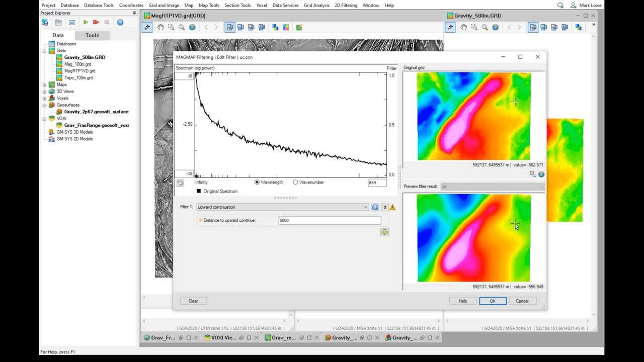
The second thing I was going to do with the gravity

[00:18:42.860]
is just produce a residual gravity

[00:18:44.820]
so that we can do some followup VOXI modeling on that.

[00:18:49.980]
So using the same menu options,

[00:18:52.150]
2D filtering, magnet filtering,

[00:18:55.500]
I’m going to use that satellite gravity,

[00:18:57.700]
500 meters, and produce a

[00:19:00.770]
regional

[00:19:03.570]
gravity grid

[00:19:06.080]
by doing an upper continuation filter on it.

[00:19:09.700]
So the same thing as what we did with the magnetics,

[00:19:11.730]
it’s still potential field data.

[00:19:13.600]
So we get…

[00:19:14.433]
We transform it back into that spectral space

[00:19:17.280]
where we would like to run these filters

[00:19:20.560]
and the upcoming continuation filter is going to

[00:19:26.090]
make a sort of a synthetic model of what that

[00:19:30.200]
density high would look like from

[00:19:32.580]
in this case 5,000 meters,

[00:19:34.370]
so that we can reduce the effects

[00:19:36.030]
of those deep crustal components on this.

[00:19:39.580]
So just press okay to generate that regional.

[00:19:43.450]
And then I’m going to have to do some grid maths

[00:19:47.230]
just briefly using grid and image with maths

[00:19:50.200]
just to remove the effect of that regional

[00:19:52.900]
and just import input our original gravity,

[00:19:55.640]
remove the regional,

[00:19:57.080]
and produce a residual grid,

[00:19:59.544]
press okay.

[00:20:01.540]
So the residual gravity now

[00:20:03.300]
will just contain those components

[00:20:05.640]
that are in that sort of that region of interest.

[00:20:09.370]
And not that those really quite deep crustal components

[00:20:13.560]
is still going quite deep in terms of scale.

[00:20:16.370]
I mean, this was a 500 meter satellite throughout that data.

[00:20:20.530]
But this is now a better defining the edges of this feature.

[00:20:24.200]
And that’s what I’d like to model.

[00:20:27.130]
So to do that, I’m going to use another tool now.

[00:20:29.000]
It’s the CET Grid Analysis.

[00:20:31.560]
And step-by-step texture ridges

[00:20:33.630]
to find the edges of that anomaly.

[00:20:37.960]
So firstly, I run a standard deviation filter to find

[00:20:41.370]
those areas where that

[00:20:44.240]
along that grid that

[00:20:45.900]
the values vary quite significantly.

[00:20:50.860]
I’ll then run a phase symmetry to highlight those features,

[00:20:55.640]
staying with the default options.

[00:21:01.590]
And then when I remove areas that are not interesting

[00:21:05.100]
using an amplitude threshold

[00:21:07.080]
to reduce that blue in that area and just highlight

[00:21:09.470]
those high amplitude features.

[00:21:16.000]
And

[00:21:17.400]
that looks pretty good.

[00:21:18.233]
So now we can go ahead and vectorize that

[00:21:20.780]
using some line thing to bring that back to just

[00:21:25.200]
straight lines that we can use in the interpretation.

[00:21:30.100]
So these lines now are completely generated from that grid.

[00:21:34.090]
I can bring in the residual gravity to compare.

[00:21:38.502]
And we can see that it’s following along the edges

[00:21:42.143]
of those features in there.

[00:21:43.120]
And also some other interesting ones

[00:21:44.750]
are added in here as well which might be of interest.

[00:21:47.490]
So I can go ahead and share that on Central as well

[00:21:50.060]
as point data or polyline data with Allan.

[00:21:53.650]
The last thing I wanted to do in Oasis montaj

[00:21:55.970]
was just to model that residual gravity.

[00:21:58.820]
And I can do that in VOXI.

[00:22:01.526]
But here I am in the VOXI menu.

[00:22:04.840]
And I’ve just bought in that regional…

[00:22:06.910]
Sorry, the residual gravity data.

[00:22:09.610]
And you can see there’s a polygon,

[00:22:12.400]
it’s clipped it’s in my topography.

[00:22:14.380]
And it’s brought in that data is points

[00:22:16.210]
located over that region.

[00:22:18.930]
VOXI allows for a number of constraints

[00:22:21.080]
that you can apply.

[00:22:22.260]
In this case, we don’t have much information yet.

[00:22:24.690]
So I’m just going to run an unconstrained inversion

[00:22:27.060]
to try and pull out 3D information that’s in this model.

[00:22:31.270]
When I press go to run inversion,

[00:22:33.720]
it uploads the data that we have in here.

[00:22:36.070]
This is the residual gravity.

[00:22:38.510]
And the mesh components that I’ve got in here

[00:22:40.700]
to Microsoft Azure

[00:22:42.530]
for that inversion to run

[00:22:44.920]
is completely encrypted.

[00:22:46.500]
And once this is uploaded and ready to go,

[00:22:49.410]
there’s no more processing on computer and I can go back

[00:22:51.930]
and do any processing and it’s not going to

[00:22:55.790]
affect the speed of the computer.

[00:22:59.410]
So I’ve already run this inversion.

[00:23:00.960]
So I might just pause this.

[00:23:02.820]
I’m going to go back to a 3D view to view that…

[00:23:06.310]
Those results.

[00:23:15.610]
And in this 3D view, I’ve got my measured residual gravity

[00:23:25.597]
shown on the top.

[00:23:26.930]
And my unconstrained inversion cube

[00:23:29.220]
or block model at the bottom.

[00:23:31.750]
I’ve also gone ahead and created some isosurfaces

[00:23:36.055]
(murmurs) can transparency there in there as well,

[00:23:38.370]
which might help with Allan’s interpretation of this.

[00:23:41.007]
You can see that there’s some angle information in there

[00:23:45.050]
which might be helpful.

[00:23:47.871]
I just want a slice on this.

[00:23:52.950]
We can see that there’s some interesting structure in there

[00:23:55.223]
that we might…

[00:23:56.150]
he might want to use

[00:23:57.760]
in that 3D modeling as well back in Leapfrog.

[00:24:00.480]
So as I go ahead and share this

[00:24:01.700]
what I can do is just right click

[00:24:03.420]
on that information I would like to share,

[00:24:06.130]
in the ProjectExplorer and upload to Central.

[00:24:18.190]
So

[00:24:19.920]
I’m going to be exporting this as an OMF

[00:24:22.230]
or Open Mining Format file.

[00:24:24.400]
OMF allows

[00:24:26.660]
sharing or point data, polyline data

[00:24:29.260]
block model data, or mesh files,

[00:24:31.610]
all packaged together in one helpful file

[00:24:34.000]
OMF file.

[00:24:35.620]
And when I share this upon Central,

[00:24:39.200]
it’s going to retain all the coordinate information

[00:24:41.970]
and for all those different types of files

[00:24:44.780]
all packaged together.

[00:24:45.750]
So it’s a really handy fall type to be sharing

[00:24:48.800]
between different teams,

[00:24:50.500]
and between different platforms as well.

[00:24:53.650]
<v Allan>Thank you so much, Mark.</v>

[00:24:55.800]
I think Mark has a left on notification for me,

[00:24:59.690]
which is located on the right side of the screen.

[00:25:03.410]
It says in here, Allan gravity, VOXI results and mag RTP.

[00:25:09.060]
Vertical derivative grids are now in the data room.

[00:25:11.730]
Pretty exciting.

[00:25:13.270]
So what I’ll do is, I’m just going to

[00:25:16.300]
go back to the projects in here,

[00:25:20.200]
and go to the data room,

[00:25:24.220]
go to the files,

[00:25:27.890]
and yeah, it’s going to gravity VOXI there over here.

[00:25:33.180]
And if I go to geophysical grids is actually

[00:25:36.840]
done the gravity residual

[00:25:39.400]
as well as

[00:25:42.220]
some mag as well I think.

[00:25:44.320]
I believe.

[00:25:45.153]
No, this are all gravities.

[00:25:46.650]
Yep. That’s fine.

[00:25:48.400]
And also in here

[00:25:51.300]
he’s done some

[00:25:52.830]
CET

[00:25:54.668]
graph and Meg limit analysis.

[00:25:57.700]
All right.

[00:25:58.830]
So what I’m going to do now is going to shift

[00:26:01.910]
the view to Leapfrog Geo.

[00:26:07.150]
The Leapfrog Geo is get the functionality

[00:26:08.730]
to download files from the data room which is from Central.

[00:26:13.100]
So what I’m going to do now is first I’m going to download

[00:26:17.360]
to the grids.

[00:26:19.910]
So under the geophysical data folder in here,

[00:26:23.980]
I can right click and I can import to the grids

[00:26:26.890]
from Central.

[00:26:28.380]
Okay.

[00:26:30.760]
And I’m going now to the

[00:26:34.580]
project, which is the

[00:26:37.460]
geophysics project that we’ve been working on.

[00:26:40.690]
Go to files folder.

[00:26:43.210]
And I’m going to go now to do fiscal grids in here.

[00:26:47.710]
And I’m going to download the gravity

[00:26:50.480]
residual grid as an example.

[00:26:53.370]
Okay.

[00:26:54.370]
I’m going to…

[00:26:55.203]
So the process for downloading the

[00:26:57.950]
magnetic RTP first vertical derivative is the same process.

[00:27:02.930]
I’m just going to show you this, just to illustrate that point.

[00:27:07.730]
And so now down in here,

[00:27:10.593]
you can now see that that’s still being downloaded.

[00:27:13.740]
Now that’s the gravity residual grid now displayed on the…

[00:27:18.030]
Under the project tree.

[00:27:19.630]
Okay.

[00:27:20.630]
Another…

[00:27:22.230]
So in order to display that they already have in here…

[00:27:26.990]
I’m going to turn off that.

[00:27:28.140]
And I’ve already

[00:27:30.430]
displayed that under the same list in here.

[00:27:32.510]
So all you need to do is to turn that on.

[00:27:35.290]
And it’s not the gravity residual grid

[00:27:38.930]
that was sent to me by Mark.

[00:27:43.250]
Another file that he has sent through

[00:27:45.080]
is the magnetic data as well,

[00:27:48.400]
which is the reduced to pole

[00:27:51.360]
first vertical derivative.

[00:27:54.510]
And clearly there’s an enhancement here

[00:27:58.390]
to look at your structural data, for example, here.

[00:28:02.660]
So just to show you, that’s the original,

[00:28:05.937]
this is the original 100 meter grid

[00:28:08.030]
and is now the process data.

[00:28:12.010]
Okay, let’s now go to importing some points.

[00:28:16.200]
So right-click input points from Central.

[00:28:22.014]
I’m going to import what

[00:28:24.290]
Mark has sent

[00:28:27.220]
when he did CET grid lineaments analysis.

[00:28:32.430]
I’m going to import, for example, the CET graph

[00:28:35.870]
CSV file

[00:28:37.610]
and click import.

[00:28:41.730]
Okay.

[00:28:42.841]
So this is the data is just an easting and northing

[00:28:46.440]
finish.

[00:28:47.980]
Okay, my elevation selected at the moment.

[00:28:50.350]
I’m just going to click continue.

[00:28:52.160]
And now that’s not the CET gravity.

[00:28:55.080]
You need to do the same process

[00:28:56.900]
for the magnetic data as well.

[00:28:59.630]
So I already have here pre-prepared

[00:29:02.940]
data.

[00:29:03.773]
So this is now my CET gravity in here.

[00:29:07.860]
And

[00:29:09.150]
my CET mag.

[00:29:12.210]
So what I’ve done for the CT gravity is

[00:29:17.000]
I have…

[00:29:17.833]
What I’ve done is I right click on this one, for example.

[00:29:22.300]
And I did a category selection,

[00:29:24.470]
’cause I don’t want be, for example, selecting all of these,

[00:29:28.620]
So I did a new category selection,

[00:29:31.820]
column is none,

[00:29:33.450]
and the name of the category selection is selection.

[00:29:38.527]
I’m just going to click okay.

[00:29:40.270]
And so what does is,

[00:29:44.380]
I’m going to select which ones in here, for example, on the

[00:29:48.600]
western part is what I’m going to use

[00:29:52.010]
to refine the mafic surface

[00:29:53.940]
that I showed you earlier on.

[00:29:55.920]
So just clicking on this one here as an example.

[00:29:59.710]
And for example, I’ve selected some of these,

[00:30:04.582]
there’s going to make this smaller make it 25

[00:30:08.090]
is the width,

[00:30:11.820]
close,

[00:30:13.810]
and I’m going to select some of these, an example,

[00:30:18.260]
and sign to create new nephrology.

[00:30:22.610]
And I’m just going to call this mafic.

[00:30:27.170]
And that is exactly what I’ve done in this process.

[00:30:30.640]
So it’s not too clear.

[00:30:31.690]
However, I can change the color to

[00:30:34.830]
something that you can clearly see.

[00:30:38.620]
So that’s not a category selection that I have done earlier.

[00:30:42.530]
So what I’ll do now is,

[00:30:44.700]
I’m going to click close in this

[00:30:46.410]
and I’m going to save this quickly.

[00:30:47.900]
However, I already have pre selected an existing one,

[00:30:53.410]
which I have done.

[00:30:54.460]
So what I’ll do is I’m going to remove this now

[00:30:59.030]
and go through with existing one

[00:31:01.070]
which is selection in here.

[00:31:03.830]
So that’s highlighted in blue.

[00:31:07.023]
And if I load my surface earlier,

[00:31:12.120]
so that’s the old surface.

[00:31:15.980]
It’s not yet honoring this particular surface.

[00:31:19.560]
So in order to honor this,

[00:31:21.170]
so what I wanted to do now is go through

[00:31:26.707]
with this surface.

[00:31:27.540]
I’m just going to show you how you can modify this.

[00:31:32.450]
Well first, because this one is already existing,

[00:31:35.050]
so it’s just going to right click in here.

[00:31:37.230]
And I just going to make a copy on this existing one.

[00:31:40.250]
So copy.

[00:31:42.470]
So I’m not dealing with the copy data which is this one.

[00:31:45.620]
So what I’ll do is right click in here,

[00:31:48.520]
and I click, I add

[00:31:50.880]
existing

[00:31:52.290]
points.

[00:31:54.300]
All right.

[00:31:55.133]
And I’m going to for example, select on those points,

[00:31:59.470]
which is this one in here.

[00:32:02.110]
And I can select, for example,

[00:32:04.410]
I’ve already created a filter which is called mafic.

[00:32:09.508]
I click okay.

[00:32:11.980]
And it’s not going to update that particular surface.

[00:32:15.980]
And if I load this now on the scene view,

[00:32:19.560]
this surface is now honoring those points

[00:32:21.980]
that the have pre-selected.

[00:32:23.860]
So that I believe that that’s one of the powers

[00:32:26.010]
of Leapfrog is to be able to make the dynamic change

[00:32:29.650]
in the surface.

[00:32:30.483]
So bringing in what Mark has sent me via Central,

[00:32:35.320]
he sent me this point and I’m going to use this points now

[00:32:38.660]
to actually modify that particular surface.

[00:32:44.250]
Let’s have a look at…

[00:32:47.090]
Let’s see if we can do something

[00:32:50.955]
on the

[00:32:53.280]
magnetic

[00:32:54.540]
data as well.

[00:32:55.390]
So I’m going to remove this

[00:32:58.768]
CET now.

[00:33:02.277]
And just viewing at this stage.

[00:33:04.070]
So I’m going to

[00:33:06.520]
turn on

[00:33:09.650]
all the liniments that Mark has sent very clear.

[00:33:13.170]
However, if I can make this gravity now transparent,

[00:33:16.710]
you can see all the liniments that Mark

[00:33:19.290]
has actually sent me via Central.

[00:33:22.357]
So clearly defining this particular…

[00:33:27.140]
This area is in here.

[00:33:29.640]
So we can see that.

[00:33:31.540]
We can assume that this bottom here are really strongly,

[00:33:37.890]
structurally control

[00:33:41.370]
as displayed in the liniment data that Mark has supplied.

[00:33:49.794]
And so just going back to

[00:33:54.210]
the surface that I have created earlier.

[00:33:57.000]
So this is not the copy data.

[00:33:59.770]
And I’m going to turn off this CET

[00:34:04.450]
point data.

[00:34:05.500]
What I’ve done in here is I’ve now created

[00:34:11.600]
a geological model database.

[00:34:16.030]
Just going to turn on that.

[00:34:18.380]
Now if I turn on

[00:34:20.540]
again my gravity data.

[00:34:25.580]
So this one shows you very sparse

[00:34:31.250]
data.

[00:34:33.130]
However, when I turned on my CET mag,

[00:34:38.430]
I think a lot has to be explained

[00:34:43.080]
in this area here.

[00:34:44.230]
So there’s a lot of,

[00:34:46.500]
probably deformity that’s happening in this area over here.

[00:34:50.730]
So what I can do is, kind of slice

[00:34:54.930]
in here.

[00:34:59.140]
I’m going to turn off my…

[00:35:00.750]
Okay, that’s the…

[00:35:04.460]
turn off that.

[00:35:10.170]
And so what I’ll do is I’m going to import

[00:35:13.670]
the data that Mark has sent me as well.

[00:35:18.580]
This is the 3D unconstrained gravity data.

[00:35:21.780]
And that will be available via OMF.

[00:35:24.120]
So there’s a functioning Leapfrog Geo,

[00:35:27.370]
just go through the Leapfrog Geo menu,

[00:35:29.630]
and go to OMF and import via Central.

[00:35:34.924]
So I’m going to go through that project again.

[00:35:39.170]
And then go to

[00:35:40.840]
this

[00:35:44.636]
VOXI

[00:35:45.469]
OMF gravity.

[00:35:47.210]
Click import.

[00:35:50.770]
Just want to show you this process.

[00:35:52.360]
I’ve already have pre imported data earlier on,

[00:35:55.670]
but I just wanted to put you to appreciate

[00:35:59.090]
what OMF functionality does in Leapfrog Geo.

[00:36:01.990]
So in Leapfrog Geo you can input both mesh

[00:36:04.900]
and the block models in here.

[00:36:07.690]
So I can actually select all of these as an example,

[00:36:12.170]
and also select the block model.

[00:36:17.250]
And then click okay.

[00:36:18.660]
So I’m not going to click okay now

[00:36:20.140]
’cause I already have an existing

[00:36:23.490]
block model in here.

[00:36:24.730]
So I’m going to click cancel now.

[00:36:27.210]
And I’m going to turn on the block model,

[00:36:30.150]
which is this one in here.

[00:36:33.330]
And at the moment,

[00:36:34.360]
so if I turn off the filter now,

[00:36:36.350]
so this is the…

[00:36:38.090]
This is the unfiltered

[00:36:42.020]
VOXI,

[00:36:42.853]
gravity VOXI.

[00:36:43.950]
So what I’m going to do now is

[00:36:45.150]
I’m going to apply out value filter on this

[00:36:48.230]
and starting from three to maximum of about 16.

[00:36:55.410]
Just kind of…

[00:36:56.760]
What I’ll do is I’m going to remove

[00:36:58.820]
this now from the scene view

[00:37:02.250]
here.

[00:37:03.083]
And what I’ll do is

[00:37:07.251]
I’m going to…

[00:37:09.920]
So this probably the surface that I wanted

[00:37:12.380]
to display earlier.

[00:37:15.070]
And this

[00:37:16.750]
has been used to guide

[00:37:19.320]
to refine this surface further

[00:37:22.130]
by just through visualization.

[00:37:24.050]
And then what I’ve done was I’ve added a few

[00:37:26.860]
structural data which I have already

[00:37:32.180]
introduced earlier,

[00:37:34.270]
which is this one here.

[00:37:36.300]
This are some of the structural

[00:37:37.610]
that I’ve added to that particular surface.

[00:37:41.760]
This…

[00:37:46.810]
Okay, so

[00:37:50.540]
if I turn off my gravity,

[00:38:09.877]
So I’m going to turn on those.

[00:38:12.760]
So basically,

[00:38:17.260]
turn on copying data,

[00:38:21.030]
structure the mesh that I’ve used earlier on.

[00:38:27.782]
So that’s the mesh that

[00:38:32.110]
has been modified based on the existing

[00:38:35.670]
3D unconstrained gravity data,

[00:38:38.130]
as well as I’ve had it a few structural data

[00:38:41.690]
at the bottom of that surface.

[00:38:48.600]
So this is just a preliminary model that I have created.

[00:38:52.860]
And I wanted to…

[00:38:54.860]
I’m interested what Mark has to say regarding

[00:38:58.580]
having to use this particular service now

[00:39:02.550]
to create a more constrained

[00:39:06.040]
gravity data.

[00:39:07.680]
So I’m interested for example,

[00:39:09.950]
in this area,

[00:39:11.420]
we have lot of structural deformity.

[00:39:13.860]
So now going back to Central and request Mark

[00:39:18.510]
to provide me with

[00:39:21.380]
a constraint gravity inversion.

[00:39:25.030]
So I’m going to go back to Central now.

[00:39:29.050]
And go back to the project earlier.

[00:39:35.330]
I’m going to reply to…

[00:39:37.890]
Go in here again.

[00:39:43.090]
And we’ll just wait for that to load.

[00:39:47.610]
And I’m going to reply to Mark,

[00:39:50.870]
Mark’s comments in there.

[00:39:56.000]
So we’ll just wait for that to load for awhile.

[00:40:00.690]
Sticking a few seconds because it’s original data set.

[00:40:05.580]
So what I’ll do in here is I’m going to notify Mark.

[00:40:11.260]
So Mark,

[00:40:13.184]
thanks for

[00:40:16.890]
providing

[00:40:20.020]
the process data

[00:40:25.820]
please

[00:40:28.160]
provide

[00:40:33.930]
constraint

[00:40:36.760]
gravity

[00:40:39.400]
inversion

[00:40:41.650]
using

[00:40:43.740]
the

[00:40:46.190]
updated

[00:40:48.100]
mafic surface.

[00:40:50.810]
So

[00:40:52.610]
I’m going to tell Mark to provide this and

[00:40:58.150]
that’s ready, the updated surface in there.

[00:41:01.050]
So what I’ll do is I’m going to

[00:41:03.910]
add a geotag

[00:41:06.710]
that’s to show him that that’s what I require.

[00:41:12.366]
And to put this in there.

[00:41:13.300]
And after that I can

[00:41:15.780]
reply.

[00:41:17.420]
So Mark’s going to receive that notification via email.

[00:41:21.340]
And is also going to be notified by this…

[00:41:26.140]
By a bell icon here.

[00:41:27.800]
And there’s also a Seequent notification

[00:41:30.140]
that he’ll be able to receive.

[00:41:31.780]
So three types notifications.

[00:41:33.900]
So he’s always on the loop

[00:41:35.580]
of what’s happening with this particular project.

[00:41:43.630]
For our summary and conclusions,

[00:41:49.500]
I go through with the first item, Mark.

[00:41:51.760]
Summary and conclusions

[00:41:52.940]
<v Mark>Yeah, absolutely.</v>

[00:41:53.773]
So we showed how Central can be used to store

[00:41:57.800]
geophysical data.

[00:41:59.330]
And that obviously there’s timestamps

[00:42:02.230]
and there’s notifications through there.

[00:42:04.730]
So there is a cloud-based system as well.

[00:42:07.110]
So it’s automatically backed up.

[00:42:09.290]
And so we showed that we can store data in a way.

[00:42:14.150]
<v Allan] >Sure.</v>

[00:42:14.983]
Just wanted to add a comment there as well.

[00:42:16.440]
It’s…

[00:42:17.273]
When you store things over the cloud, it’s also safer.

[00:42:21.250]
It saves in real time and allows for stakeholders

[00:42:24.180]
to share the latest versions.

[00:42:27.120]
Secondly, just going through that

[00:42:30.620]
updated data is not readily available.

[00:42:33.270]
Mark comment on Oasis montaj.

[00:42:35.850]
<v Mark>Yeah.</v>

[00:42:36.683]
I guess so in the past,

[00:42:37.770]
the geophysics would be

[00:42:39.880]
to creating that data in birding

[00:42:41.300]
and enhancing and then maybe sharing by Dropbox or FTP.

[00:42:46.005]
So in this way, we can just upload straight from OEM,

[00:42:49.120]
from a Oasis into Central.

[00:42:51.900]
And Allan can be notified straight away to access that data.

[00:42:54.750]
So it’s pretty quick and fast

[00:42:57.620]
to get that and share that data.

[00:43:00.850]
<v Allan>Okay, I’ll go through with a third one.</v>

[00:43:02.360]
So geoscience teams need to work more closely together.

[00:43:05.330]
So basically, we need to get teams sharing data

[00:43:09.440]
and projects in real-time

[00:43:12.040]
and also in 3D environment.

[00:43:13.720]
It’s actually very important as well.

[00:43:15.750]
And Leapfrog can actually pull the geophysics data

[00:43:18.840]
from Central and use this to build models

[00:43:21.560]
and target anomalies in 3D space.

[00:43:24.970]
So the Central notification lets you keep

[00:43:28.410]
in touch with what’s happening in the projects.

[00:43:31.820]
You’re actually…

[00:43:32.690]
You’re basically, actively working on.

[00:43:35.540]
And there are notifications from events

[00:43:38.280]
that can be received by email or via Central portal as well.

[00:43:44.000]
And lastly,

[00:43:47.490]
we can accelerate the running of the multiple

[00:43:50.810]
3D scenarios or models.

[00:43:52.470]
So Oasis montaj is the desktop application

[00:43:56.340]
coupled with VOXI earth modeling,

[00:43:58.440]
which is a cloud application

[00:44:01.980]
for geophysical inversion

[00:44:03.240]
can quickly run multiple models or scenarios.

[00:44:07.240]
And

[00:44:08.890]
Mark has clearly illustrated earlier

[00:44:12.110]
that he can share this data readily in Central

[00:44:15.300]
for peer review and notifications.

[00:44:17.640]
And then

[00:44:19.520]
myself earlier, I was able to import all of the data

[00:44:23.433]
that he has uploaded to Central,

[00:44:25.970]
so that I can integrate this with other geoscience data

[00:44:30.430]
for ongoing 3D modeling interpretation.

[00:44:34.880]
And also I’ve requested Mark lastly earlier on

[00:44:39.520]
that I can…

[00:44:40.720]
He can work on my existing Leapfrog mesh,

[00:44:43.170]
which is the mafic surface that I was working on.

[00:44:47.230]
And he can use this to constraint geophysical inversions

[00:44:50.550]
in Oasis montaj.

[00:44:55.580]
So for our next Technical Tuesday workshop,

[00:44:58.780]
it’s on the 27th of April.

[00:45:02.110]
It’s about Drillhole Data Tips for Leapfrog.

[00:45:05.330]
I hope that everyone will end this session

[00:45:08.600]
at the moment can attend this online.

[00:45:11.280]
And this is

[00:45:13.717]
how to properly set up your drillhole database

[00:45:16.640]
in Leapfrog before modeling.

[00:45:20.410]
So other resources that will be helpful

[00:45:22.410]
is please log into our secret website,

[00:45:26.040]
Seequent.com.

[00:45:27.230]
Or if you want to do additional learning

[00:45:30.030]
about Oasis montaj or Leapfrog,

[00:45:32.450]
you can log into, myseequent.com

[00:45:36.760]
for additional resources.

[00:45:38.930]
And if you want training or project assistance,

[00:45:42.940]
then you can always contact your local team.

[00:45:47.090]
If you want to talk to someone at the technical support,

[00:45:50.760]
please get in touch with them through [email protected].

[00:45:55.040]
Thank you so much for your time guys.

[00:45:57.370]
I really appreciate for your time to attend this webinar.

[00:46:00.860]
Mark, you want to say a few words?

[00:46:02.970]
<v Mark>Yeah, great.</v>

[00:46:03.803]
I hope that all the geophysicist out there

[00:46:06.390]
found something useful and being able to share your data

[00:46:08.510]
with the geology teams in that way.

[00:46:10.290]
And maybe there’s some hints and tips

[00:46:12.970]
that could be used over the next few days.

[00:46:15.930]
<v Allan>Thank you so much.</v>

[00:46:16.763]
<v Mark>Thank you.</v>

[00:46:17.596]
<v Allan>Bye for now.</v>