Technical Tuesday: Getting Started with Leapfrog Edge – Useful preparation tips before you start your next project.

With Leapfrog Edge you can dynamically link to your geological model and perform all the key steps to prepare a resource estimate and validate the results. The webinar will focus on the major benefits of using Leapfrog Edge and what concepts to consider before you start.

Join Seequent’s Jelita Sidabutar (Project Geologist) and Steve Law (Senior Project Geologist) who will discuss:

• What is Leapfrog Edge and why is it beneficial to your work processes.
• Preparation Tips – Validate your data.
• The importance of domaining – the link between your Geology Model and the Resource Estimate.
• Estimation Strategies.

Please note, this webinar will be run in a combination of Bahasa and English

Overview

Video Transcript

[00:00:01.513]
<v Jelita>(speaking in foreign language)</v>

[00:09:49.300]
I’m now handing over to you, Steve.

[00:09:51.130]
Thank you very much.

[00:10:01.160]
<v Steve>Thank you Jelita for that introduction.</v>

[00:10:04.610]
The next section we will cover the concepts

[00:10:07.600]
that we should consider whilst creating a resource estimate.

[00:10:11.760]
At the same time, we will see

[00:10:14.600]
and demonstrate the capability of Leapfrog Geo

[00:10:17.970]
and Leapfrog Edge.

[00:10:20.810]
The first section I’d like to look at

[00:10:22.350]
is preparation of your data.

[00:10:25.100]
This includes viewing and visualizing our information,

[00:10:29.210]
checking that it’s in the correct spatial location

[00:10:31.860]
and understanding the impact of missing or no values.

[00:10:41.180]
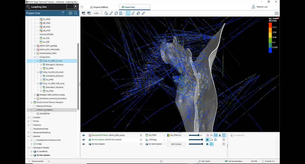
This model represents an epithermal gold underground mine.

[00:10:44.840]
We have a series of underground

[00:10:46.960]
and surface drill holes

[00:10:48.600]
and a geological model has been developed

[00:10:51.830]
with several different load structures.

[00:10:55.730]
The first thing we should do is check that spatially,

[00:10:58.340]
relates to things such as typography

[00:11:01.460]
and underground development.

[00:11:07.284]
You can see here that the colors of the drill holes

[00:11:09.060]
all seem to go to the surface and don’t go above it.

[00:11:14.540]
And if we have a look underground,

[00:11:22.930]
We can see that the drill fans of underground

[00:11:26.500]
do seem to match up with the underground drill (indistinct)

[00:11:29.980]
that are being mapped in by survey.

[00:11:33.420]
So that’s a good starting point.

[00:11:38.320]
We can run a series of statistical evaluations

[00:11:41.750]
to check our data.

[00:11:43.730]
The first part of that is looking at our data as a whole,

[00:11:46.680]
before it has been domained.

[00:11:48.840]
I will look at the gold data set for this.

[00:11:52.890]
Leapfrog has a function

[00:11:54.700]
to be able to check errors on loading.

[00:11:57.090]
You’ll see here that over here

[00:11:58.560]
in the drill whole essay table,

[00:12:00.690]
there are little red indicators on each of the elements

[00:12:03.820]
except for gold.

[00:12:05.800]
Each of these means we should check and we have a function

[00:12:10.210]
at the database table level called fixed errors.

[00:12:17.150]
If I click on the gold, this one is been reviewed,

[00:12:20.300]
which is why there is no little red symbol,

[00:12:22.960]
but what it shows us is that in the data set,

[00:12:25.850]
it will show us any missing information.

[00:12:28.100]
And also any below detection values.

[00:12:30.880]
These could be less thans or negatives,

[00:12:33.240]
or just default values.

[00:12:37.380]
We can decide whether we want to omit missing information

[00:12:40.960]
or replace it with a different value.

[00:12:43.530]
So in this case, we’re omitting missing data,

[00:12:46.750]
but we’ve got some negative 0.01, 0.02, 0.05,

[00:12:52.750]
and we have the capability of giving a different rule

[00:12:56.470]
for each one.

[00:12:57.990]
Otherwise if we don’t define

[00:13:00.240]
a value for each different figure,

[00:13:02.570]
it will just replace all of them with 0.001.

[00:13:08.240]
Once these rules have been put in place,

[00:13:10.490]
we tick this little box up here and hit the save button.

[00:13:14.170]
And then that will apply going forward.

[00:13:17.070]
If we reload our data,

[00:13:18.440]
those same rules will be still in place.

[00:13:20.800]
You don’t have to do it each time you change your data set.

[00:13:25.340]
You would then go through and do the same thing

[00:13:28.440]
for the other elements.

[00:13:30.540]
As we’re not using those today.

[00:13:32.857]
I don’t need to do that.

[00:13:35.000]
There is always a default value.

[00:13:36.690]
So in this case, I’m omitting missing data.

[00:13:41.770]
And in this case,

[00:13:43.100]
keeping positive values would be the default.

[00:13:45.250]
If you didn’t come to do that.

[00:13:46.880]
So ideally we would always generally want to replace

[00:13:50.750]
non-positive values so that they don’t cause issues

[00:13:56.570]
in the underlying statistics.

[00:13:59.630]
When we hit save, then it processes those changes.

[00:14:05.940]
We can also look at a histogram.

[00:14:08.470]
If we look at a histogram of gold by itself,

[00:14:11.430]
underlying statistics,

[00:14:14.580]
we can see a histogram of the data.

[00:14:19.480]
And we can see that there are no negatives.

[00:14:22.450]
So everything is zero at the minimum.

[00:14:24.830]
And we’ve got…

[00:14:25.663]
Gives us an idea on the scale of our data.

[00:14:28.190]
So this goes up to 443 grams per ton.

[00:14:33.825]
Leapfrog histograms are interactive with the scene.

[00:14:37.290]
So as long as I’m displaying this table in the scene,

[00:14:41.310]
if I wanted to see where all of my values

[00:14:43.590]
above one gram were, I can highlight my histogram

[00:14:49.290]
and in the scene view,

[00:14:55.250]
I can see that they’re all values above one.

[00:14:59.530]
So this is just a filter

[00:15:01.280]
that’s applied interactively on the scene.

[00:15:04.090]
It’s not one that we can save.

[00:15:06.580]
I come back to here.

[00:15:08.060]
I can turn the histogram off and all my data will come back.

[00:15:16.760]
Generally though,

[00:15:17.593]
we’re wanting to look at a domain level for our statistics.

[00:15:22.040]
So in this case,

[00:15:23.540]
we’ve got a vein system that’s been developed

[00:15:27.460]
in the geological models.

[00:15:34.690]
And I also have built a geological model

[00:15:37.670]
where I’ve split the veins into separate pieces.

[00:15:40.600]
With (indistinct) based from the underlying vein system.

[00:15:44.190]
So that if I update my veins here,

[00:15:46.420]
that will flow through automatically to this section.

[00:15:53.900]
So I can evaluate any geological model

[00:15:57.980]
back to my drill holes.

[00:15:59.340]
It’s basically flagging the codes into the drill hole space.

[00:16:02.980]
We do that by right clicking on the drill holes

[00:16:08.550]
and doing a new evaluation.

[00:16:11.090]
That then lets us pick a geological model

[00:16:13.460]
and it creates a new table.

[00:16:15.580]
In this case down here, estimation domains, evaluation.

[00:16:21.100]
I’ve then merged that using the merge table function

[00:16:24.210]
with the essay table,

[00:16:25.890]
and then I’m able to do statistics on that.

[00:16:30.050]
So I’ll do a box plot.

[00:16:33.570]
And this will show me the global…

[00:16:40.310]
The gold broken down by domain.

[00:16:43.050]
So we can see here that four of them have similar values,

[00:16:48.340]
but then 4,400 is a lower grade vein.

[00:16:51.280]
That has a mean somewhere below one gram.

[00:16:55.460]
Sorry, of around two grams.

[00:17:07.920]
We also can do compositing within Leapfrog Geo.

[00:17:14.638]
This is all done underneath the new numeric composite.

[00:17:18.000]
And what we’re able to do is we can do it against

[00:17:20.330]
the subset of codes.

[00:17:22.250]
And this allows us to choose in this case,

[00:17:26.370]
our estimation domains.

[00:17:28.650]
And at the same time, we can do compositing

[00:17:32.260]
for all the different domains.

[00:17:34.390]
And we could choose to do all of the elements.

[00:17:39.280]
At the same time.

[00:17:41.220]
We can apply different rules to each domain.

[00:17:44.370]
In this case, I want to use the same rules,

[00:17:47.590]
but if I had a domain where I wanted to use

[00:17:51.320]
2 meter composites, rather than 10 meter composites,

[00:17:54.000]
I could do that here.

[00:17:55.400]
Now in the real ones that I’ve done,

[00:17:58.820]
we are looking at one meter composites

[00:18:03.260]
across all the domains.

[00:18:06.100]
And if I have less than half a meter remaining

[00:18:09.260]
of when it hits the domain boundary,

[00:18:11.720]
then it’s going to distribute the piece

[00:18:13.550]
across the whole domain.

[00:18:15.940]
We have a concept here called minimum coverage.

[00:18:19.520]
This really only has an impact if we have missing data.

[00:18:22.910]
If there is no missing data

[00:18:24.300]
and you’ve got values throughout your mineralization zone,

[00:18:27.730]
that does not matter what you put in here.

[00:18:30.420]
The default value is 50%.

[00:18:32.990]
And generally you either choose 0%, 50% or 100%.

[00:18:40.900]
We have a really useful tool called drill hole correlation,

[00:18:46.320]
where you can examine the results of your compositing

[00:18:49.470]
and get a feel for how changing those different parameters

[00:18:52.850]
might affect the composites.

[00:18:55.894]
So I have a look at this one.

[00:18:57.570]
I’ve picked a particular hole.

[00:18:59.350]
Now this one had some missing data down

[00:19:02.610]
in the middle of one of the veins.

[00:19:04.540]
So if I wanted to have a look and see

[00:19:06.230]
what the different compositing would do,

[00:19:08.580]
so that it’s all one meter.

[00:19:10.310]
That the only change is that the coverage has been changed

[00:19:13.440]
from 0, 50 to 100.

[00:19:16.120]
And basically the percentage means

[00:19:18.130]
it’s relative to the length that you’ve chosen.

[00:19:23.660]
So if we just zoom in a little bit.

[00:19:43.430]
Okay, so if we have a look at down here,

[00:19:45.750]
there’s a gap in our data in through here.

[00:19:49.000]
With 0 and 50% coverage,

[00:19:51.920]
we still get a composite being placed in through here.

[00:19:56.203]
You can see here that that 1.7

[00:20:01.683]
has been taken over into the composites.

[00:20:05.880]
But if we use 100%,

[00:20:07.240]
which basically means that I need a full one meter

[00:20:10.490]
to be keeping it,

[00:20:11.710]
then it’s not keeping that last one meter piece.

[00:20:16.520]
The other thing we can look at in this scenario too,

[00:20:19.510]
is have we done our domain correctly?

[00:20:22.200]
This one down here is clearly using this 11.25.

[00:20:26.980]
And in the original essays,

[00:20:28.270]
it’s obviously a combination of the 18.5

[00:20:32.780]
and some of this 0.36 has been included.

[00:20:36.170]
But we have a 97 gram essay interval

[00:20:39.490]
and that’s composited to 58

[00:20:41.570]
and it’s not included in the vein.

[00:20:44.030]
So that may be a misinterpretation at this level.

[00:20:47.490]
Well, maybe it’s another vein

[00:20:49.240]
that’s not being modeled at this stage.

[00:20:51.860]
But it’s just one way of looking at your data

[00:20:55.340]
and determining have you…

[00:20:57.650]
Is the interpretation honoring the data as best as it can.

[00:21:04.810]
These correlation tables can be all saved.

[00:21:07.950]
So you can have multiple of these saved as drill hole sets

[00:21:11.570]
under the drew hall correlation folder in through here.

[00:21:18.450]
The next stage in running our resource estimate

[00:21:21.570]
and equally is important as the data integrity

[00:21:25.290]
is the importance of domaining.

[00:21:27.840]
And this is the link between your geology model

[00:21:30.580]
and the underlying estimate.

[00:21:32.970]
And we have a series of tools

[00:21:34.930]
where we can do exploratory data analysis.

[00:21:40.160]
Leapfrog Geo and Edge relies on having

[00:21:44.380]
a robust geological model at that underlies the estimate.

[00:21:49.250]
When we are using Leapfrog Edge,

[00:21:51.330]
we have an estimation folder and within that,

[00:21:55.030]
we create a new domain estimation.

[00:21:59.950]
I’ve already got a series of them created here.

[00:22:02.670]
So we’re going to have a look at the estimation

[00:22:05.980]
for vein for 201.

[00:22:12.430]
So the domain is chosen from at a closed mesh

[00:22:17.150]
within the system.

[00:22:18.100]
So it can be anywhere in the meshes folder

[00:22:20.810]
or ideally within a geological model.

[00:22:25.370]
We can then pick up our numeric values

[00:22:27.960]
and they can either be from the underlying essay data,

[00:22:31.810]
and then we can composite on the fly.

[00:22:34.490]
Which is what I’ve done in here.

[00:22:36.210]
Or if we chose to use one of the composited files,

[00:22:39.240]
which are here,

[00:22:40.380]
then that compositing section would gray out.

[00:22:46.230]
The first thing it shows us is a…

[00:22:50.620]
Take that back to (indistinct).

[00:22:52.580]
Is a contact plot.

[00:22:54.610]
And this shows us the boundary conditions of the domain

[00:22:57.400]
and against what’s immediately outside it.

[00:23:01.000]
So we’re looking and right angles to our domain

[00:23:03.690]
in all directions.

[00:23:05.030]
And it’s showing us here that within one meter

[00:23:10.500]
of the inside, we’ve got high values.

[00:23:13.530]
So we’re getting higher essays above 10 grams per ton.

[00:23:17.080]
But immediately crossing the boundary.

[00:23:19.260]
We’ve dropped down to below five grams per ton.

[00:23:22.700]
Now some of these things could be modeled in other veins.

[00:23:25.710]
So we’re really just looking around the immediate contact.

[00:23:29.980]
If there is a sharp drop-off such as this,

[00:23:32.730]
then it suggests that we should use a hard boundary.

[00:23:35.820]
If not, we will use a soft boundary,

[00:23:38.890]
which allows us to use some of the samples outside

[00:23:42.380]
up to a certain distance, which we define

[00:23:44.920]
to be included in the estimate.

[00:23:48.330]
We are still only estimating within the domain itself,

[00:23:51.230]
but it’s using some samples from outside.

[00:23:54.990]
Now, how do we choose the domain?

[00:23:57.170]
There are lots of things to consider

[00:23:58.920]
and the domain, it can be the most important part

[00:24:02.680]
of your resource estimate.

[00:24:04.480]
If we get the geological interpretation wrong,

[00:24:07.920]
then our underlying estimate will be incorrect as well.

[00:24:12.350]
So some of the things that we should consider,

[00:24:15.080]
what is the regional and local scale geology like?

[00:24:18.920]
Do we have underlying structural controls?

[00:24:23.400]
There are different phases of mineralization

[00:24:25.890]
and are they all the same style?

[00:24:29.125]
At least some of it,

[00:24:30.290]
could there be early stage pervasive mineralization

[00:24:33.330]
cut across by later structurally focused

[00:24:37.040]
mineralized stones.

[00:24:39.487]
Faults and defamation.

[00:24:41.980]
How do these impact?

[00:24:43.240]
Are they syndepositional with the mineralization?

[00:24:46.410]
Are they all post or later and are cutting things up?

[00:24:52.460]
The continuity of the mineralization

[00:24:54.310]
and this flows through, into our variography studies.

[00:24:59.340]
Do we have very short scale continuity

[00:25:02.960]
such as we often get within gold mines?

[00:25:05.780]
Or is there a better continuity such in base metals

[00:25:09.120]
or ion ore.

[00:25:14.570]
Have there been over printing effects

[00:25:16.270]
of alteration and weathering?

[00:25:18.040]
Have we got super gene enhancement of the mineralization

[00:25:21.280]
up above the base of oxidation?

[00:25:27.900]
So Leapfrog Edge relies on having a closed volume

[00:25:30.400]
as the initial starting point.

[00:25:33.520]
We develop a folder for each of these

[00:25:36.750]
and we can look at the domain in isolation.

[00:25:40.530]
So we’re looking here at a single vein.

[00:25:44.200]
We can look at the values within that vein.

[00:25:49.280]
And we can do statistics on those.

[00:25:53.610]
Continue graphs.

[00:25:59.660]
So again, this is domain statistics now,

[00:26:02.410]
so we can see that we still have a skewed data set.

[00:26:06.580]
So ranging from 0.005, up to 116.5 grams.

[00:26:14.200]
The mean of our data is somewhere around 15.

[00:26:19.530]
If we wanted to consider whether we need to top cut,

[00:26:22.800]
we can first look and see where those values are.

[00:26:28.500]
So we can see here that there’s a few scattered values

[00:26:36.270]
within the domain.

[00:26:38.220]
They’re not all clustered in one area.

[00:26:40.370]
So if they are all clustered down, say down here,

[00:26:43.070]
then we might have to consider subdividing those out

[00:26:45.940]
as a separate little high grade domain.

[00:26:49.620]
But they’re not so unlikely to do that.

[00:26:51.900]
So another option is to look at top cutting.

[00:26:55.660]
One till we have for looking at top cutting

[00:26:57.890]
is the low probability plot.

[00:27:00.070]
Is there a space where the plot

[00:27:04.660]
starts to deteriorate or step.

[00:27:07.470]
Up here, we can see around about 90 grams.

[00:27:11.420]
There’s a cut up above that 98.7th percentile.

[00:27:18.060]
We could be a little bit more conservative

[00:27:20.220]
and come down towards 40 grams.

[00:27:24.960]
Down through here.

[00:27:26.780]
There’s no right or wrong on this.

[00:27:28.940]
And you would actually run the estimate

[00:27:31.170]
potentially at both top cuts and see how much impact

[00:27:36.110]
removing some of this high grade has

[00:27:38.280]
from the underlying estimate.

[00:27:45.800]
Within each domain estimation,

[00:27:48.060]
we have the ability to do variography studies

[00:27:50.920]
under the spacial models folder.

[00:27:53.520]
We can apply variable orientation.

[00:27:55.710]
So if our domain is not linear and we can see here

[00:27:59.680]
that this vein does have some twists and turns in it,

[00:28:04.670]
then we can use variable orientation,

[00:28:06.640]
which will align the search ellipsoid to the local geometry

[00:28:10.670]
to get a better sample selection.

[00:28:14.010]
And we can also consider de-clustering

[00:28:16.820]
under the sample geometry.

[00:28:19.260]
De-clustering is often when we are drilling a resource

[00:28:23.980]
from early days through the ground control.

[00:28:26.560]
In the early days,

[00:28:27.410]
we’ll start finding bits and pieces of higher grade,

[00:28:30.930]
and we tend to close our drills facing up

[00:28:33.420]
towards where the high grade is.

[00:28:35.740]
This could have the tendency of vicing

[00:28:38.530]
our drilling towards the high grade.

[00:28:40.770]
So the overall mean of the data in this instance

[00:28:43.840]
could be 15 grams (indistinct).

[00:28:48.620]
But the underlying real grade of that

[00:28:51.540]
could be a little bit less than that

[00:28:52.980]
because we haven’t actually drilled

[00:28:54.750]
all of the potentially low grade areas

[00:28:57.120]
within that domain.

[00:29:01.160]
So we can set up a sample geometry.

[00:29:06.150]
If I open up this one.

[00:29:08.020]
And what I’ve done here is I’ve aligned the ellipsoid

[00:29:13.500]
roughly with the geometry of the vein.

[00:29:17.930]
And I’ve looked at 40 by 30 by 10 meters.

[00:29:22.330]
This data set has a lot of drilling.

[00:29:25.490]
It’s got underground, great channel samples as well,

[00:29:29.820]
ranging from three meters apart.

[00:29:32.060]
And we can get up to 40 or 50 meters space,

[00:29:34.930]
drill holes in some areas as well.

[00:29:37.400]
So thinking about maybe if I indicated range was 40 meters,

[00:29:43.860]
I will see whether there’s an impact from de-clusttering.

[00:29:46.860]
A little graph here suggests that there is,

[00:29:49.250]
we’ve got an input mean of 14.96.

[00:29:53.430]
But the de-clustered mean suggests

[00:29:56.386]
that it’s closer to 14.

[00:29:59.840]
What’s the impact of making my spacing a little bit larger?

[00:30:03.100]
If I have a look at 80 meters,

[00:30:07.620]
I can see that potentially getting something

[00:30:11.090]
of a similar result.

[00:30:14.920]
To see what the de-clustered mean is

[00:30:17.000]
I can do the properties.

[00:30:19.480]
So I can see that my naive mean is 14.966.

[00:30:24.520]
And my de-clustered mean is 14.23.

[00:30:27.970]
If I look at slightly wider spacing,

[00:30:30.570]
my de-clustered mean is going up to 15,

[00:30:33.070]
but it’s very close to the naive mean.

[00:30:35.920]
So this suggests that overall,

[00:30:38.000]
there may be a little bit of impact of de-clustering,

[00:30:41.210]
but my overall grade

[00:30:42.780]
is definitely somewhere between 14 and 15 grams.

[00:30:45.980]
It’s not 12, it’s not 16 or 17.

[00:30:50.140]
In Leapfrog Edge you do have the opportunity

[00:30:52.400]
to apply de-clustered weights,

[00:30:55.480]
which this defines for each of these

[00:30:58.120]
during running an inverse distance estimator.

[00:31:03.420]
Often though I won’t use it directly

[00:31:05.440]
and just consider how it looks at the end.

[00:31:07.980]
When we’re looking at the statistics of our block model,

[00:31:10.880]
I’m hoping that the overall domain statistics of my blocks

[00:31:14.950]
will be similar to the de-clustered mean.

[00:31:17.610]
So if I get a bit of a variance

[00:31:19.900]
and instead of being close to 15, it’s closer to 14.

[00:31:23.360]
I wouldn’t be concerned.

[00:31:24.920]
But if I were getting a block estimate

[00:31:26.740]
of well about 15, say 15 and a half 16 overall,

[00:31:31.320]
or down around 13,

[00:31:32.850]
I’m either underestimating or overestimating

[00:31:35.830]
on a global scale.

[00:31:38.710]
And in that case I may need to change

[00:31:41.500]
some of my estimation search parameters.

[00:31:48.903]
One of our biggest tools of course, is variography.

[00:31:52.230]
We do have the capability of transforming our data.

[00:31:56.200]
So this is done generally for skewed data sets

[00:32:00.640]
and it helps us calculate a semi variogram

[00:32:04.720]
that’s better structured

[00:32:06.660]
than if we do not transform the values.

[00:32:10.460]
We simply right click on our values and transform them.

[00:32:13.900]
And that gives us the transformed values here.

[00:32:16.970]
If we look at the statistics of the transform values,

[00:32:21.390]
they simply are a log normal histogram.

[00:32:26.080]
So all the impact of the higher grades

[00:32:28.200]
is being compressed down into the tail.

[00:32:30.820]
So when we calculate our variogram

[00:32:32.890]
we’re not getting such wide variations between sample pairs.

[00:32:37.800]
And this gives us a better structured variogram to model.

[00:32:43.130]
If we have a look at the variogram for this one,

[00:32:54.300]
we are able to have the radial plot.

[00:33:00.230]
Now this radial plot is in the plane of the mineralization.

[00:33:04.000]
So we tend to set the plane up first.

[00:33:06.490]
And in this case it’s aligned with the underlying vein.

[00:33:13.500]
And then we model in the three directions

[00:33:15.710]
perpendicular to that.

[00:33:18.652]
The range of greatest continuity

[00:33:21.950]
is reflected by the red arrow.

[00:33:24.140]
And then the cross to that is the green.

[00:33:27.720]
And then across the vein itself,

[00:33:29.820]
the smallest direction is represented in the blue.

[00:33:33.570]
These graphs are interactive with the scene.

[00:33:36.360]
So we can always see our ellipsoid in here.

[00:33:39.850]
And if we move that it will move to the graphs.

[00:33:44.170]
Again, if we change this one here,

[00:33:50.210]
it will correspondingly change the ellipsoid

[00:33:53.130]
so we can see we’ve stretched it out in that orientation.

[00:33:57.480]
So we’ll take that back to where it should be.

[00:34:01.350]
Down through here.

[00:34:03.332]
We can see that my ellipsoid has as shrunk.

[00:34:05.780]
So we can always keep in contact

[00:34:08.150]
without our geology and our orientations

[00:34:10.900]
and make sure we don’t inadvertently

[00:34:12.800]
turn out ellipsoid in the wrong direction.

[00:34:18.330]
The modeling tools are all standard,

[00:34:20.610]
similar to what’s available

[00:34:22.840]
in most variogram modeling packages.

[00:34:26.160]
You can adjust your lag distance, your number of lags,

[00:34:29.180]
angular tolerance, and bandwidth as needed.

[00:34:34.360]
Once we’ve got a model that may fit,

[00:34:38.240]
we save it and we back transform it.

[00:34:40.850]
So the back transform is automatic.

[00:34:43.030]
Once we hit that button and takes us

[00:34:45.010]
from that normal score space back into our graded space,

[00:34:49.710]
before we run the estimate.

[00:34:52.860]
We can save any number of different variograms.

[00:34:58.180]
So I can actually copy this variogram here.

[00:35:01.700]
I can make some slight changes to it

[00:35:03.940]
and choose to use that one.

[00:35:05.697]
And I could run multiple variograms

[00:35:08.100]
and test to see what kind of impact they may have.

[00:35:16.220]
Up until this point we’ve been focusing

[00:35:18.090]
mainly on our diamond drilling information

[00:35:21.370]
that we’ve got for this particular domain.

[00:35:24.500]
Leapfrog now has the capability

[00:35:26.270]
of storing multiple databases within the project.

[00:35:29.810]
So I’ve got a diamond drill hole database,

[00:35:32.840]
and I’ve also got a grade control

[00:35:35.110]
underground channel database.

[00:35:39.190]
I can choose to have a look at the impact

[00:35:43.450]
between, is there a bias between the channels

[00:35:46.250]
and the drill holes.

[00:35:49.600]
At the moment, we need to export these

[00:35:51.830]
and join them together as points.

[00:35:54.150]
In an upcoming release, we will be able

[00:35:56.340]
to merge these things automatically.

[00:35:59.620]
Here I have one meter composites

[00:36:01.190]
of the diamond drill holes and the channels.

[00:36:03.780]
And if I do statistics on that, I can run a QQ plot.

[00:36:10.210]
I’ve used query filters to isolate the diamond drill holes

[00:36:14.120]
and the channels.

[00:36:15.590]
And we can see here that there is a bias

[00:36:18.770]
to the underground channels in turn,

[00:36:20.810]
that they tended to give higher grades

[00:36:24.220]
than the equivalent located diamond drill holes.

[00:36:28.380]
So that’s something to be keep in mind.

[00:36:32.670]
This is a real mind, and that was definitely the case.

[00:36:36.710]
And we had to consider applying different top cuts

[00:36:41.680]
to the channel samples versus top cuts

[00:36:43.940]
to the underlying diamond drill holes.

[00:36:46.840]
To help reconcile with the mill.

[00:36:49.950]
It’s a lot easier to tackle that kind of situation.

[00:36:54.560]
When you start getting production data.

[00:36:56.960]
Before that, you don’t really know whether channels

[00:37:01.430]
are more representative

[00:37:02.760]
than all the diamond drill holes are.

[00:37:09.960]
Again, we can look at that data.

[00:37:14.720]
So here we have our channel samples in there as well.

[00:37:18.140]
So we can choose to use all of that information

[00:37:21.440]
within our estimate.

[00:37:25.840]
We can run variograms with both data sets combined.

[00:37:29.260]
We can run it with just the channels

[00:37:30.950]
or with just the diamond drill holes

[00:37:32.780]
and see whether there is any influence

[00:37:35.610]
on the variography on the different types of data

[00:37:38.610]
that we’re using.

[00:37:41.410]
To understand whether there’s any impact

[00:37:43.340]
on adding channel samples into it

[00:37:45.330]
for the variography,

[00:37:46.740]
we can simply copy the entire folder.

[00:37:50.239]
We replace the underlying information

[00:37:54.211]
with the combined data set, which is through here.

[00:37:57.600]
And we can still see that there’s still

[00:37:59.550]
quite a big drop in the contact plots

[00:38:02.570]
and no real changes in the pattern there.

[00:38:05.900]
Our variogram for the drilling only

[00:38:09.609]
gave us quite short ranges, 25 to 15 and 4 across the vein,

[00:38:14.900]
which we were able to model

[00:38:15.990]
with a single exponential structure.

[00:38:18.760]
If we have a look at the transformed variogram again

[00:38:23.080]
for that combined channel data.

[00:38:34.440]
We can see that it’s quite similar.

[00:38:38.299]
So the sills changed a little bit.

[00:38:40.490]
It didn’t really have to change the ranges.

[00:38:42.650]
So it’s giving a similar result in both cases.

[00:38:54.280]
Once we have done our data analysis,

[00:38:56.320]
we’re ready to set up our estimation strategy.

[00:39:00.920]
There are various things that we consider.

[00:39:03.300]
What stage are we at in the project?

[00:39:06.120]
Are we in early exploration or pre mining stages,

[00:39:09.640]
or are we at grade control level?

[00:39:11.880]
If we’re a great control level,

[00:39:13.180]
we’re going to have a lot more information and data.

[00:39:16.268]
We may well be dealing with shorter ranged information

[00:39:20.080]
that we’ve got.

[00:39:21.130]
Whereas in the early stages, we don’t really know.

[00:39:24.490]
We might not have enough information to do kriging

[00:39:28.240]
or get a valid variogram.

[00:39:29.640]
In which case we may decide to use inverse distance

[00:39:32.940]
to some power.

[00:39:36.970]
The search strategy is an important concept.

[00:39:40.400]
And sometimes it can have more impact than the variogram

[00:39:43.890]
that we are working with.

[00:39:46.430]
There are lots of different theories

[00:39:48.080]
on what kind of search parameters we should set up.

[00:39:52.550]
Should we use lots of samples with long distances?

[00:39:55.750]
Should we use a small number of samples

[00:39:58.610]
to try and better match local conditions,

[00:40:02.320]
especially in grade control that can often be the case.

[00:40:05.890]
So it might use limited number of samples

[00:40:07.723]
over shorter search ranges.

[00:40:10.690]
There’s also the potential to use multi pass strategy.

[00:40:14.880]
Where you will use a larger number of samples

[00:40:17.357]
over a short distance to better reflect the local.

[00:40:20.490]
But then you still need to estimate blocks further away

[00:40:24.200]
and you will gradually increase the search distance.

[00:40:28.500]
And at the same time, you may or may not

[00:40:30.520]
change the number of samples.

[00:40:32.520]
If you’re trying to estimate far-flung blocks

[00:40:35.680]
with limited data,

[00:40:36.860]
well, then you’re going to have to have

[00:40:37.930]
a low number of samples, but a large search.

[00:40:42.830]
The issue with this too, though,

[00:40:44.590]
is you can get artifacts between the search boundaries.

[00:40:48.770]
Classic is where you will display the results,

[00:40:51.630]
and you can see the concentric ring of that grade

[00:40:54.660]
around each search limit.

[00:40:56.570]
So we don’t want to see that kind of thing.

[00:40:58.740]
So we would need to do something

[00:41:00.720]
to try and eliminate that kind of thing.

[00:41:07.765]
Kriging Neighborhood Analysis

[00:41:09.210]
is a way of testing a whole series of our variables.

[00:41:13.590]
Lowest number of samples, maximum number samples,

[00:41:16.290]
minimum number of samples.

[00:41:18.280]
Trying different search distances.

[00:41:22.066]
Discretization, another parameter that we could play with.

[00:41:25.380]
That depends more on our ultimate block size in our models.

[00:41:30.170]
All of these things can be tested quite easily with Edge

[00:41:33.290]
and it’s all really a matter of copying estimators

[00:41:37.400]
and then running them through.

[00:41:40.060]
We have a separate webinar that goes through this strategy.

[00:41:46.670]
We can set up either inverse distance,

[00:41:49.390]
nearest neighbor or kriging estimators.

[00:41:53.460]
We also have the ability to do

[00:41:55.150]
radial basis function estimator,

[00:41:57.190]
which is the same algorithm that is used in the modeling

[00:42:00.580]
and in the numeric models in Leapfrog Geo.

[00:42:03.470]
It is more of a global estimate and you don’t necessarily…

[00:42:07.150]
It’s not too bad to use if it’s difficult

[00:42:09.400]
to apply a variogram.

[00:42:12.640]
We’re going to focus on the kriging estimated today.

[00:42:16.750]
So to create a new one,

[00:42:18.380]
you just right click and got a new kriging estimator.

[00:42:24.920]
If you have one already set up like this,

[00:42:27.020]
you can choose either whether it’s ordinary or simple

[00:42:32.300]
and we deploy our discretization here.

[00:42:34.570]
And that’s generally related to our block size.

[00:42:38.530]
Any variogram that’s stored in the folder

[00:42:40.590]
can be selected from here.

[00:42:42.860]
And if we want to apply top cuts on the fly,

[00:42:47.730]
we can click the values at this point.

[00:42:49.840]
And this will apply only to this particular domain.

[00:42:55.310]
The most important part is setting up our…

[00:43:00.870]
Cancel that one.

[00:43:02.557]
It’ll open up when it’s already there,

[00:43:07.810]
is setting up our search.

[00:43:09.620]
Now, in this case, I’m using variable orientation,

[00:43:11.990]
but initially you would set it to the underlying variogram.

[00:43:16.890]
This is 4.281, and that will take in the orientation

[00:43:22.750]
and it takes the maximum ranges that you developed.

[00:43:25.810]
But you can choose to make this smaller,

[00:43:29.820]
or you can make them bigger.

[00:43:31.440]
It’s up to you.

[00:43:32.840]
If we use variable orientation,

[00:43:34.610]
which is using the local geometry of the vein in this case

[00:43:37.930]
to help with the selection, we simply tick that box here.

[00:43:41.720]
We do have to have a variable orientation set up.

[00:43:46.071]
In the search parameters,

[00:43:47.410]
obviously we’ve got the standard ones.

[00:43:49.430]
We’ve got minimum and maximum number of samples,

[00:43:52.290]
we can apply an outlier restriction.

[00:43:55.070]
This is more of a limited top cut.

[00:43:57.620]
So in this case, we could have applied an overall top cut

[00:44:01.310]
that may take out all the values, say above 100,

[00:44:05.360]
but then what we’re doing is saying that if we’re within 40%

[00:44:09.820]
of the search, that’s defined here,

[00:44:13.840]
then we will use the value.

[00:44:16.640]
And then if it’s further than that away,

[00:44:19.120]
we will start to cut that down.

[00:44:20.880]
So in this case, we’re using 60.

[00:44:23.640]
We can apply sector searches on a quadrant or opt-in basis.

[00:44:28.150]
And we have drill hole limit, which is maximum samples,

[00:44:30.950]
per drill hole.

[00:44:32.060]
Which is relating back to here.

[00:44:34.260]
So in this case it means we’d need at least two drill holes

[00:44:38.980]
to make an estimate.

[00:44:41.840]
So on our early passes,

[00:44:43.990]
we may have quite a few restrictions in,

[00:44:46.840]
but as we loosened it up,

[00:44:48.180]
if we’re doing a multi-pass strategy,

[00:44:50.430]
we may need to vary that down and take some of those away.

[00:45:03.390]
In this project, at this stage,

[00:45:04.910]
if we’re only looking at the diamond drill only set up,

[00:45:07.800]
we’ve got a domain destination for vein for 201,

[00:45:11.200]
and we’ve also created another one for vein 4,400.

[00:45:15.720]
Within those, we’ve got two passes of kriging

[00:45:19.540]
and I have got a inverse distance.

[00:45:21.940]
One to set up as a comparison.

[00:45:24.140]
And underneath the 4,400 domain

[00:45:27.080]
we have a three pass kriging setup.

[00:45:29.970]
And again, I’ve got an underlying

[00:45:31.550]
in the first distance to set up

[00:45:33.470]
as a comparison to the kriging.

[00:45:37.310]
We want to be able to join all this information together

[00:45:39.640]
at the end.

[00:45:40.473]
So we have a thing known as a combined estimator.

[00:45:44.070]
This is set up at the top level here, combined estimator.

[00:45:48.380]
And it’s like a merge table with the drill holes.

[00:45:51.440]
If we have a look at this one here.

[00:45:54.364]
What this is doing, it’s joining together the domains

[00:45:57.790]
so that we’ll be able to see both domains at the same time

[00:46:00.970]
in the scene and then it’s got the passes.

[00:46:03.550]
And it’s important that the passes are in order.

[00:46:06.390]
So pass one and two.

[00:46:08.280]
One, two, three.

[00:46:09.800]
The way Leapfrog works is that for each pass it reruns

[00:46:13.890]
and flags a block with a value for every block.

[00:46:17.660]
So you will get subtle differences

[00:46:19.730]
between pass one and pass two in some of the blocks.

[00:46:24.240]
This is telling it that if I get an estimate

[00:46:27.220]
on the first pass, then I will use it.

[00:46:30.970]
But if not, then I will use pass too.

[00:46:33.980]
If I haven’t estimated that block

[00:46:35.950]
after pass one or pass two with this phone,

[00:46:39.050]
then it will take the value for pass three.

[00:46:41.840]
And then the final value is displayed

[00:46:44.050]
using this combined variable name here.

[00:46:47.950]
At the same time that we’re storing this information.

[00:46:52.020]
It will flag for us what pass

[00:46:54.780]
that the estimate occurred on.

[00:46:56.640]
So that is this EST estimated here.

[00:47:04.780]
All of these parameters can be viewed in a parameter report.

[00:47:12.540]
And this gives us a nice table that shows us, for instance,

[00:47:15.820]
all the different search parameters

[00:47:17.640]
for each of the estimation domains that we’ve set up.

[00:47:20.780]
We can see our ellipsoid ranges.

[00:47:23.470]
This is a good way of checking everything overall

[00:47:25.690]
to see whether we might’ve made a mistake.

[00:47:28.090]
For instance, did we…

[00:47:30.710]
If there was a maximum value that has been set incorrectly,

[00:47:34.350]
if there is an issue here,

[00:47:35.710]
we can just simply click on that there

[00:47:38.910]
and it’ll open up the underlying estimator for us.

[00:47:42.650]
And we could go back and change that to another value.

[00:47:47.090]
It’s interactive.

[00:47:48.460]
So as soon as I changed the value here,

[00:47:51.010]
you’ll see that the table will update.

[00:47:54.710]
In the next release, this table itself

[00:47:57.050]
will be directly editable,

[00:47:58.800]
but for the moment it just opens up the underlying form.

[00:48:02.320]
So I’ll just change that back to 24.

[00:48:10.432]
And that’s done.

[00:48:11.990]
So you can see there that it’s reprocessing

[00:48:14.130]
there in the background, but we can still do things.

[00:48:17.470]
We can export this data to a spreadsheet,

[00:48:26.200]
and it’ll give you a overview of that.

[00:48:30.860]
It’s a formatted spreadsheet.

[00:48:32.610]
So that’s easy to take all this information

[00:48:35.700]
and put it into a report.

[00:48:37.330]
So here, I’m looking at the variogram tab.

[00:48:39.460]
So it’s giving me the name, the variants, the nugget,

[00:48:43.090]
the sills, and our ranges.

[00:48:44.900]
So all neatly tabulated, ready to put into a report.

[00:48:52.620]
Once we have set up all of our estimation parameters,

[00:48:56.410]
we are ready to work with our block model.

[00:49:00.250]
So in this case, I’m using a sub-block model

[00:49:05.520]
and we have a new format called Octree.

[00:49:08.150]
Which is similar to (indistinct) structure.

[00:49:12.730]
Basically it means that if we have a parent size,

[00:49:15.810]
then the sub-block size must be a multiple of two.

[00:49:19.490]
So 1, 2, 4, 8 up to 64 divisions of the parent block.

[00:49:25.930]
We can rotate in dip and as in any block model.

[00:49:30.450]
When we’re constructing our models,

[00:49:32.200]
we can see relative to our data.

[00:49:36.930]
I bring back in some of my values, for instance, here.

[00:49:45.620]
Bring in the drill holes.

[00:49:49.870]
So we just construct a single block model

[00:49:51.830]
for all of this data.

[00:49:53.700]
We can change the boundary at any time using the handles.

[00:49:58.380]
It shows us our sub-block size, as we zoom in there.

[00:50:03.630]
So these are the parent blocks and these are the sub-blocks.

[00:50:10.650]
It automatically triggers on anything

[00:50:12.750]
that we bring across to the side.

[00:50:15.540]
So here I’m wanting to store my host drop model,

[00:50:18.830]
my vein system and my estimation domains.

[00:50:21.990]
So each thing here will basically flag a corresponding block

[00:50:25.610]
with the codes.

[00:50:27.270]
And then I’m bringing across my estimators.

[00:50:30.540]
Now for final results, I only actually need

[00:50:33.440]
the combined estimator in here.

[00:50:35.880]
But if I want to validate against the swath plot

[00:50:38.190]
and have a look at the underlying composites,

[00:50:40.490]
I do need to bring across the original estimator itself.

[00:50:46.010]
Because this is where the information is stored

[00:50:48.710]
on what samples are being used and distances,

[00:50:52.020]
and average distance, et cetera.

[00:50:56.210]
This is simply taking the end result of each estimate

[00:50:59.800]
and flagging it into the block.

[00:51:03.660]
We also have the capability of flagging meshes

[00:51:07.450]
directly into the block model now.

[00:51:09.460]
And this is under a function called combined meshes.

[00:51:17.800]
That is done down here

[00:51:22.280]
in the combined models folder.

[00:51:25.620]
And it’s actually a grouped mesh.

[00:51:27.710]
I’ve done a grouped mess for the drives.

[00:51:30.240]
So I open that up.

[00:51:31.637]
All we need to do is select the meshes

[00:51:34.390]
directly from the meshes folder.

[00:51:37.110]
So I’ve added plus.

[00:51:39.160]
That will let me go.

[00:51:40.650]
In this case, I’ve got design stored as designs.

[00:51:45.040]
And I’ve got development drives in the meshes.

[00:51:47.630]
So any valid closed solid within the project

[00:51:52.940]
inside a geological model,

[00:51:54.510]
meshes folder or designs folder can be used.

[00:51:59.280]
It will automatically pick up the name

[00:52:01.950]
that’s been assigned to that object.

[00:52:04.240]
And this can be changed if you wish to change it.

[00:52:07.230]
And then that will be flagged.

[00:52:10.470]
Then evaluate it into your model

[00:52:13.080]
and then this will be evaluated.

[00:52:15.840]
So I’ll just kill that.

[00:52:19.500]
So to look at the results of our block model,

[00:52:21.430]
we just drag it into the scene.

[00:52:31.580]
And all the options of viewing,

[00:52:33.400]
all the different variables that we’ve stored down here.

[00:52:36.787]
The one really good one that we’ve got is looking at status.

[00:52:41.240]
So if we wanted to have a look at our inverse distance

[00:52:45.170]
of that vein 4,400, and we went and looked

[00:52:48.010]
at the status of that.

[00:52:50.830]
If I turn off outside, it shows me that the set up

[00:52:57.390]
I’ve got for the search.

[00:52:58.730]
The white blocks are estimated

[00:53:01.840]
and the purple ones have not been estimated.

[00:53:04.460]
So I may want to do a second pass to fill in these blocks.

[00:53:14.280]
If we look at the combined variable, for instance for

[00:53:17.323]
AU 4,400 and go to the est parameter.

[00:53:27.644]
(indistinct) essays.

[00:53:30.830]
It will color code the passes for us.

[00:53:34.810]
So we can see here that the blocks

[00:53:36.640]
that were estimated on the first pass are the pale blue.

[00:53:40.770]
Slightly darker blue for the second.

[00:53:42.850]
And for the third.

[00:53:44.320]
If I evaluate, if I highlight one of those blocks,

[00:53:47.800]
I can see here that the first pass,

[00:53:50.440]
I’ve got a value of 5.59 on the past two, it was 5.96.

[00:53:58.280]
A little bit different.

[00:53:59.520]
And then the third one looking at a much larger search

[00:54:02.840]
and less samples, it’s come up with 4.093.

[00:54:06.270]
But because we got I value on the first pass,

[00:54:09.330]
then the underlying end result is that first pass.

[00:54:14.530]
If we click on the second pass here,

[00:54:17.200]
we can see that there was no value assigned on pass one.

[00:54:21.520]
So it’s going to use the value from pass two,

[00:54:24.500]
which is 5.51.

[00:54:27.090]
You can see that’s the same vein down in here.

[00:54:30.220]
So we can get a good idea of how much of our resource

[00:54:35.810]
is being estimated on each pass.

[00:54:38.950]
We can quantify that within the block models.

[00:54:42.980]
We have the ability to build a series of reports

[00:54:47.470]
and they are stored within the block model.

[00:54:49.720]
So when any data is updated and the rebuttal reruns,

[00:54:53.850]
the reports will rerun for us.

[00:54:56.300]
So if I have a look at this estimation passes 4,400,

[00:55:07.160]
I can see that on the first pass,

[00:55:10.230]
this was the volume of blocks estimated,

[00:55:13.160]
then pass two and pass three.

[00:55:15.510]
So it’s approximately a little bit over 50%

[00:55:18.947]
was done on pass one.

[00:55:21.180]
I can also check the volume of the blocks

[00:55:23.940]
against the volume of the underlying wire frame,

[00:55:26.990]
because we want them to be fairly close to each other.

[00:55:29.610]
So in this case the block volume is total 574,000.

[00:55:35.100]
And if we have a look at the domain volume, it is 583.

[00:55:44.260]
So we’re within a couple of percent of each other.

[00:55:48.280]
If we wanted to try and get it closer,

[00:55:50.220]
we would have to change our block size

[00:55:52.180]
and make it potentially smaller.

[00:56:00.900]
So after getting a feel

[00:56:02.150]
for what’s happening without estimation.

[00:56:05.240]
Obviously we want to have a look at our actual results.

[00:56:09.570]
And the best way of course

[00:56:11.430]
is to visually compare our goal values

[00:56:20.700]
against our underlying sample values.

[00:56:24.770]
And we would need to use the same color scheme.

[00:56:32.318]
(indistinct) those, so.

[00:56:41.950]
Look at a thin slice.

[00:56:59.550]
So it would bring in our values and our block model

[00:57:01.603]
with the same color scheme,

[00:57:03.590]
and then look through it and check the overall

[00:57:06.780]
down the line colors of the samples

[00:57:09.980]
is matching the colors of the blocks.

[00:57:12.520]
Where they’re dominantly low grade in this case, green,

[00:57:15.550]
the blocks are green up in here.

[00:57:17.727]
But as we go into higher grade areas,

[00:57:20.730]
we can see that the blocks it’s starting to change color.

[00:57:26.840]
Another way of validating our data

[00:57:28.600]
is to look at swath plots.

[00:57:30.260]
Again, these are built within the block model themselves,

[00:57:33.390]
so we can apply as many swats plots as we wish.

[00:57:36.800]
And once they’re built, they’re stored.

[00:57:38.780]
So if we want to re-look at the one built

[00:57:41.010]
for swath 4,400,

[00:57:45.610]
we can see here that I’m comparing…

[00:57:48.069]
In this case, I am looking at inverse distance

[00:57:50.680]
against kriging for pass two.

[00:57:54.770]
And the underlying composites are highlighted in red.

[00:58:02.180]
In this case.

[00:58:03.320]
So the underline composites are red and the two estimates.

[00:58:06.840]
We can see that the kriging and the inverse distance

[00:58:10.670]
are very similar to each other.

[00:58:12.820]
It’s in the Y direction, Z direction.

[00:58:17.110]
We will often see this where we want the trend

[00:58:19.320]
to be followed.

[00:58:20.770]
And they estimate tends to bisect the highs and lows

[00:58:24.600]
where there’s an abrupt change from high to low.

[00:58:31.230]
But overall, the trend is being followed.

[00:58:34.070]
And that suggests that this is a reasonable estimate.

[00:58:39.130]
The other way, of course,

[00:58:40.300]
is to look at the actual statistics.

[00:58:43.130]
So we can do that on the block model statistics.

[00:58:47.940]
We can do a table of statistics.

[00:58:55.260]
We would pick out categories.

[00:58:57.430]
So in this case, if I select my estimation domains,

[00:59:07.380]
None there, and we’ve done 4201, 4,400.

[00:59:18.110]
And then we need to pick the values.

[00:59:20.280]
So in this case I will look at the combined variable.

[00:59:25.860]
So we can see here that the mean for 201 is 15.3.

[00:59:30.647]
And the mean of the blocks for 4,400 is 2.085.

[00:59:35.770]
If we remember, we can go back to the domain

[00:59:39.570]
and look at the statistics of 4201.

[00:59:43.421]
The mean there is 14.7.

[00:59:48.290]
So just a little bit under 15 and for the other one,

[00:59:58.800]
it is 2.65.

[01:00:04.200]
So again, a little bit lower in that case,

[01:00:07.100]
a little bit higher, a little bit lower.

[01:00:09.110]
And then we may want to tweak some of the parameters

[01:00:11.480]
to see if we can get that little bit closer.

[01:00:13.700]
But luckily in the area where we’re mining,

[01:00:16.270]
it might make perfect sense.

[01:00:17.900]
And there may be some Edge effects

[01:00:19.990]
that causes the global mean

[01:00:21.550]
to be not quite exactly what you’d expect.

[01:00:24.280]
But it’s important to validate the block’s statistics

[01:00:28.210]
against the sample statistics.

[01:00:31.700]
The final thing we can look at then is the report

[01:00:34.310]
from the block model.

[01:00:35.670]
So we can again create reports

[01:00:40.630]
built within the block model itself.

[01:00:43.170]
We’ve got one already checked here.

[01:00:45.210]
So if we select different categorical columns

[01:00:49.510]
in this case, building estimation domains.

[01:00:54.810]
And whether or not it’s mined

[01:00:57.190]
based on underlying stope and development drives

[01:01:00.410]
and I’m reporting against a final goal field.

[01:01:04.430]
All this is, is the combined variable

[01:01:07.610]
and any blocks that weren’t estimated after the three passes

[01:01:11.080]
were assigned a very low value.

[01:01:14.410]
So that will give us the table.

[01:01:17.290]
So we can see for each of the estimated domains,

[01:01:21.080]
we’ve got divided up into development and stope panels,

[01:01:24.720]
and what’s been left un-mined.

[01:01:26.920]
And the results.

[01:01:30.250]
And at this stage this is applied at a cutoff.

[01:01:32.910]
We can store any number of these in there as well.

[01:01:39.040]
So I hope that that has been informative

[01:01:42.020]
on things to consider when looking

[01:01:45.260]
and running a resource estimate.

[01:01:49.804]
(mouse clicking)

[01:01:59.210]
So support is available at all times from our Perth office.

[01:02:03.680]
Our headquarters is in New Zealand in Christchurch.

[01:02:06.690]
And [email protected] is the best place to locate us,

[01:02:11.280]
and get ahold of us.

[01:02:14.800]
Thank you very much for listening to the presentation today.