Target for ArcGIS Pro 2.2 – Enhancements for better visualization and interpretation of drillhole data

This webinar is the best place to learn how the new functionalities can improve efficiency in your workflows, give you more flexibility and help you make decisions faster.

Webinar highlights include:

• Map Scale in Section View
• Offset Symbology in 2D Maps
• New Drillhole Planning Mode – Target and Trace
• Strip Logs
• And more!

Overview

Video Transcript

[00:00:00.770]<v ->Hi, welcome to Target for ArcGIS Pro 2.2 release Webinar.</v>

[00:00:06.680]My name is Kanita Khaled,

[00:00:08.100]and I’m a geophysicist at Seequent,

[00:00:10.160]based in our Toronto headquarters in Canada.

[00:00:14.010]In this release webinar,

[00:00:15.270]I’ll give you a quick tour of the latest features coming up

[00:00:18.150]in Target for ArcGIS pro.

[00:00:20.840]With this release,

[00:00:21.673]we’ve continued to add new enhancements and improvements

[00:00:24.920]when visualizing your subsurface,

[00:00:27.070]and Drillhole Data.

[00:00:29.030]We listened to the features that you’re looking for

[00:00:31.040]in the product and added them to our priority list.

[00:00:35.350]We hope that with these new features and improvements,

[00:00:37.780]your team can generate meaningful

[00:00:39.455]and valuable data products to improve your exploration

[00:00:43.110]and project workflows.

[00:00:45.960]I’m particularly excited to introduce to you

[00:00:48.220]a few new features, which I’ll demonstrate in this video.

[00:00:51.710]I’ll also be sharing with you,

[00:00:53.250]tips on how to use these features for yourself.

[00:00:58.870]Our latest release feature focuses on a few key areas,

[00:01:02.078]your requests, things that you mentioned

[00:01:04.590]that you’d like to see in the product,

[00:01:06.840]new or enhanced functionalities that we believe will

[00:01:09.606]take your workflow to the next level,

[00:01:13.050]overall usability and experience,

[00:01:17.580]and the latest version of Target for ArcGIS Pro,

[00:01:20.470]will support desktop versions ArcGIS Pro 2.5 and also 2.6.

[00:01:30.070]Before we get started,

[00:01:31.260]I’d like to bring your attention to a few valuable resources

[00:01:34.490]that are available to you with your subscription,

[00:01:36.900]to Target for ArcGIS pro.

[00:01:41.950]By logging onto my.seequent.com,

[00:01:45.130]you’ll be able to access knowledge articles,

[00:01:47.447]help files and learning paths

[00:01:50.300]related to Target for ArcGIS pro.

[00:01:53.309]The features and functionalities covered in this video

[00:01:56.570]will also be covered in more detail in the online

[00:02:00.627]learning content, under learning, online learning,

[00:02:04.512]and then Target for ArcGIS pro.

[00:02:13.246]All right, let’s take a quick look at the agenda for today.

[00:02:16.980]Symbology improvements,

[00:02:18.490]we will start off with looking at some

[00:02:20.610]of the symbology improvements that are new

[00:02:22.640]to Target for ArcGIS pro.

[00:02:24.940]These improvements will allow you to offset symbology

[00:02:27.760]away from the drill trace as well as view numerical data

[00:02:32.050]such as assay as bar plots along the Drillhole trace.

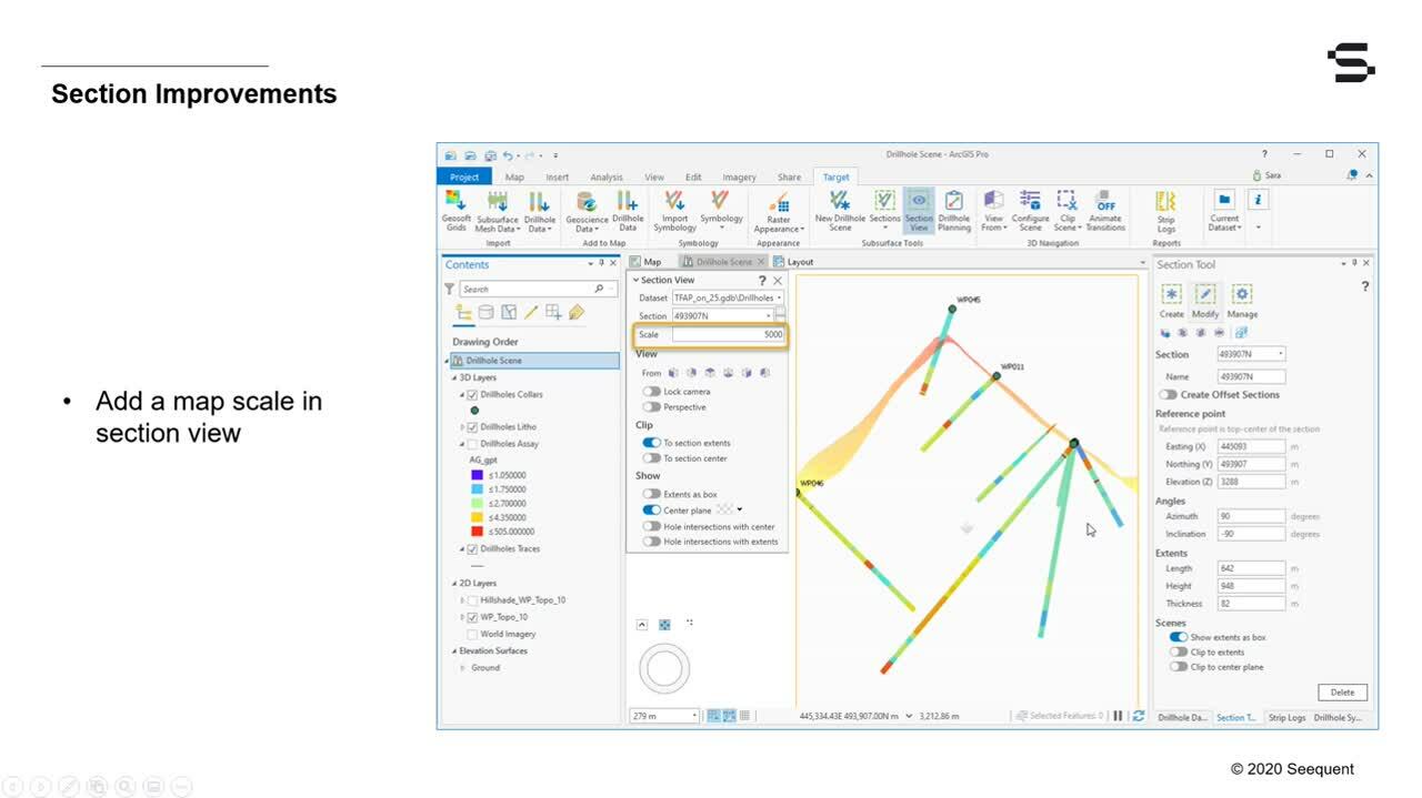
[00:02:37.540]Section improvements,

[00:02:39.810]we have made section improvements such as adding map skills

[00:02:42.730]to section views.

[00:02:46.150]New Drillhole Planning Mode,

[00:02:47.990]we added a new Drillhole planning mode that allows you

[00:02:50.970]to specify the planned end of hole location and the angle

[00:02:55.930]of approach so that the ideal color location

[00:02:58.670]can then be calculated.

[00:03:00.720]I’ll walk you through how this can be done.

[00:03:04.920]Last but not least, Strip Logs.

[00:03:07.000]Strip Logs or graphical drill logs are now an available

[00:03:10.600]functionality in Target for ArcGis Pro.

[00:03:13.580]You can use Strip Logs to graphically visualize multiple

[00:03:16.410]Downhole drilling attributes to see better correlation

[00:03:19.290]in your Drillhole Dataset.

[00:03:24.170]Our first topic is Symbology Improvements.

[00:03:27.370]The obstinate symbology feature in Target for ArcGis Pro

[00:03:31.420]is a simple, yet very powerful tool for visualizing

[00:03:34.310]multiple data types together along

[00:03:36.640]the same Drillhole traced.

[00:03:42.030]Visualizing multiple data sets together such as a major

[00:03:46.380]or a minor rock type along the same Drillhole trace

[00:03:50.260]allows your team to draw further insights about your data.

[00:03:54.640]This capability allows you to visualize multiple data types

[00:03:57.848]along the same Drillhole,

[00:03:59.660]enabling correlation and better interpretation workflows.

[00:04:04.470]In addition to adjusting the size of the symbology for

[00:04:08.560]numerical data, you can also specify an offset amount

[00:04:13.048]away from the Drillhole trace.

[00:04:17.185]This allows you to stack multiple attributes or data types

[00:04:21.560]on either side of the Drillhole trace allowing for

[00:04:25.120]much easier correlation.

[00:04:28.630]Let’s go ahead and demonstrate this within the application.

[00:04:33.062]Okay, so here I have our GIS pro loaded with my project

[00:04:37.721]topography.

[00:04:39.630]I also have signed into my my secret account,

[00:04:42.598]and now it can see my target toolbar.

[00:04:46.630]I’m going to go ahead and add in my Collar Data,

[00:04:51.970]and my Drillhole trace, and then zooming in,

[00:04:54.250]I can see that those elements are now visible,

[00:04:57.250]my Collars and my trace.

[00:05:00.127]If I wanted to go ahead and add in a few more of the

[00:05:03.723]attributes that are available within the data set,

[00:05:06.650]I would head over to this ‘Add to Mac group’

[00:05:10.690]and then select Drillhole data.

[00:05:13.690]And from here,

[00:05:15.290]I can see the list of all of the different types of

[00:05:18.610]attributes that are available for this Drillhole data set.

[00:05:22.380]I primarily have From/To Data available for this data set.

[00:05:29.576]I’m going to expand out my Lithology group here,

[00:05:33.040]and I can see the various types of Lithology attributes

[00:05:36.669]that are present within this data set.

[00:05:38.987]I’m going to turn on the Rock Type,

[00:05:44.550]and once I turned that on that I can see my Rock Type

[00:05:48.060]visualized on my scene here,

[00:05:51.660]and primarily it’s a Dolomitic Siltstone or a Sandstone.

[00:05:57.340]If I want to visualize another attribute such as

[00:06:00.670]the alteration or the geochemistry,

[00:06:03.010]I can go ahead and turn those elements on as well.

[00:06:06.810]So for example,

[00:06:08.140]if I were to head over to alteration and I can see that I

[00:06:11.620]have multiple types of alterations logged

[00:06:15.130]for this data set, alteration type, degree, et cetera.

[00:06:19.016]Let’s go ahead and turn on this primary alteration,

[00:06:24.800]and I can see wasn’t locked for all of the Drillholes,

[00:06:27.250]it was locked for some of them, but where it is lines,

[00:06:30.360]I can see that that alteration is actually being displayed

[00:06:33.680]right on top of the Lithology.

[00:06:35.400]So if I click those on and off from my content,

[00:06:38.210]I can see they’re overlaying right on top of each other.

[00:06:43.210]This is an okay way to look at my data and correlate

[00:06:47.450]my data, but it would be a lot easier if they were

[00:06:50.870]offset away from each other so that I could correlate them

[00:06:53.560]a little bit better.

[00:06:55.950]To do this, I’m going to head over to the Symbology tab

[00:07:00.647]here.

[00:07:04.610]And because I had this selected,

[00:07:06.940]this is the field that is currently shown under

[00:07:13.520]the color field, and I’m coloring these by categories,

[00:07:16.710]and I can see here that there is now an

[00:07:19.010]offset option available,

[00:07:21.660]and I can type in a number here to offset this attribute

[00:07:27.370]away from the Drillhole trace.

[00:07:29.130]So let’s go ahead and try 5,

[00:07:33.370]And yep, I can see that that attribute has now shifted over

[00:07:37.109]to the right side of that Drillhole trace,

[00:07:39.410]I can increase that a little bit more,

[00:07:43.300]and in a similar manner, I can select the Lithology,

[00:07:47.018]and I can see that the Symbology color field here just

[00:07:50.730]switched because I had just selected this color,

[00:07:53.560]and I can offset this to,

[00:08:00.328]minus 10 away

[00:08:02.370]from the Drillhole trace,

[00:08:03.780]so the other side of my Drillhole trace,

[00:08:06.710]and now I can see both of the attributes, very easy to see,

[00:08:11.150]very easy to correlate, side-by-side.

[00:08:14.540]I can take this a level further if I wanted to,

[00:08:17.610]so let’s say I wanted to go ahead and add in yet another

[00:08:21.210]Drillhole data type,

[00:08:25.390]we could potentially add,

[00:08:27.900]let’s say we wanted to add the grain size, for example.

[00:08:34.010]And again, I can see that the grain size is being visualized

[00:08:37.350]right along the Drillhole trace here,

[00:08:40.642]so now I’m visualizing three different attributes at the

[00:08:43.950]same time.

[00:08:44.890]If I wanted to, I could go ahead and offset that a specific

[00:08:48.270]amount as well,

[00:08:49.520]and of course you can add as many different fields as you’d

[00:08:52.820]like to visualize as makes sense for your interpretation

[00:08:56.774]process.

[00:09:01.890]Okay, so we’ve taken a look at how to visualize an offset

[00:09:05.050]categorical data like Lithology, Alteration,

[00:09:07.997]Grain size, et cetera.

[00:09:10.250]What about numerical data?

[00:09:12.520]We can do this as well.

[00:09:13.950]So one really effective way of visualizing

[00:09:16.710]numerical Drillhole datasets is by using bar plots.

[00:09:21.110]Let’s try that out.

[00:09:22.470]I’m going to go ahead and turn off some of these attributes

[00:09:26.680]that are currently on my scene here.

[00:09:29.560]Okay, scene is empty, just the colors and the traces.

[00:09:33.070]I’m going to go ahead and go back to the ‘Add to Map’ group

[00:09:36.240]and then Drillhole data.

[00:09:39.350]And this time I want to add in some of the numerical data,

[00:09:42.760]like my day here under Geochemistry.

[00:09:47.210]And the first thing I want to try is my lead zinc total

[00:09:52.520]amount here and press apply.

[00:09:55.860]And I can see that those values are then centered along

[00:10:00.720]my trace, just like it was with the categorical data.

[00:10:05.280]And so similar to before we can go back to Symbology

[00:10:11.427]and we can specify an offset amount.

[00:10:14.820]But before I do that, I want to customize a Symbology,

[00:10:18.810]not just to color by values, but also by size.

[00:10:25.210]We’re going to select color and size by values to do that.

[00:10:29.610]And we have a few new fields now available to fill in.

[00:10:35.500]So my color field is automatically lead zinc

[00:10:39.800]and the size field I’m also going to change

[00:10:42.300]to lead zinc total.

[00:10:44.060]So both color and size is then affected by

[00:10:47.300]the lead zinc field.

[00:10:51.040]The minimum size here, I’m going to set to five

[00:10:56.180]and the maximum size here, let’s do 75 and let’s press apply

[00:11:01.580]to see how that looks.

[00:11:04.520]We’re still centered along our trace, but now we can see

[00:11:07.740]a more of a histogram style look,

[00:11:11.100]this is a really effective way to kind of at a quick glance,

[00:11:15.530]see where my high values are and where my low values are

[00:11:18.640]because not just visualizing what the colors you’re also

[00:11:21.810]visualizing and categorizing by the numerical values present

[00:11:27.170]in that dataset.

[00:11:29.230]Okay.

[00:11:30.100]What if I’m wanting to offset this? I could do that as well.

[00:11:34.200]I could also align this to either side

[00:11:37.290]of the Drillhole trace.

[00:11:39.950]So let’s go ahead and align to the right side,

[00:11:47.640]and that would align this particular attribute

[00:11:51.280]to the right side,

[00:11:52.550]and I still have the ability here to offset,

[00:11:56.150]let’s try five,

[00:12:01.970]or negative five actually.

[00:12:07.640]There we go.

[00:12:08.473]So now I’m offset negative five to the right side

[00:12:12.030]of my Drillhole trace.

[00:12:14.660]This makes it easier for me to add in yet another Symbology.

[00:12:20.100]So let’s go back here,

[00:12:21.987]I’m going to add in my silver this time,

[00:12:25.640]and I can see it centered again,

[00:12:28.660]along my trace.

[00:12:31.170]So let me go back into my Symbology and instead of

[00:12:36.380]this uniform, color and size look,

[00:12:38.860]I’m going to try and color by size and by values.

[00:12:47.820]And I’m going to choose both my color and size field to be

[00:12:51.550]silver,

[00:12:54.460]using a similar minimum, maximum size,

[00:12:57.390]I’m going to use five and then let’s try a hundred here

[00:13:05.000]then let’s align that to the left side.

[00:13:13.510]And of course you do have the ability to offset.

[00:13:22.270]That way your page is a little bit cleaner here,

[00:13:26.560]your scenes are little bit neater,

[00:13:28.350]and you can zoom around your scene here,

[00:13:31.553]and I can now try to correlate a little bit better.

[00:13:35.330]Let me go to a Drill trace that’s little bit

[00:13:37.090]more interesting here.

[00:13:38.480]So for example, this Drillhole trace,

[00:13:40.560]I have my lead zinc to the right side,

[00:13:44.080]and my silver to the left side,

[00:13:46.090]and I can now start to make relations that yes,

[00:13:49.240]where I have my higher showings of silver,

[00:13:51.870]I potentially also have higher showings of lead and zinc.

[00:13:55.840]So this leads to a much more effective

[00:13:58.310]interpretation process.

[00:14:03.070]Switching now from my 2D map to my 3D Drillhole scene,

[00:14:08.720]I can see these side by side.

[00:14:12.240]Lets drag in the Topography from the 2D map

[00:14:18.950]into my 3D scene here, so I can better,

[00:14:22.438]orient myself.

[00:14:26.422]There we go, there’s my 3D scene with my Topography

[00:14:31.692]and I can visualize this offset Symbology feature

[00:14:36.080]in a similar manner in the 3D view or the categorical data

[00:14:41.219]where I have visualized my Lithology data,

[00:14:44.412]along the Drill trace in 3D,

[00:14:47.630]and I’m also able to apply an offset and where I have data

[00:14:52.130]available I can visualize multiple categorical data sets

[00:14:56.680]side by side in a 3D manner in my Drillhole scene.

[00:15:02.700]Section Improvements.

[00:15:05.490]All features that you see on cross sections are

[00:15:08.471]modeled representations of the real world.

[00:15:12.673]Being able to see and change the scale of a section is

[00:15:16.510]really important to give the audience a sense of size of

[00:15:19.730]scale when you’re viewing these features in a section map.

[00:15:26.460]Target for ArcGis Pro 2.2 now includes the ability to be

[00:15:31.290]able to add a map scale when visualizing a section

[00:15:36.210]or user map scale when visualizing a section.

[00:15:39.720]When the cross section is viewed in section view

[00:15:43.840]with this tool right here,

[00:15:45.450]the map skill feature can then be used to view the automatic

[00:15:49.730]scaling of each section as the program has selected,

[00:15:53.780]but also be able to manually specify the scale value for

[00:15:57.990]yourself.

[00:15:59.280]Let’s take a quick look at this in the application.

[00:16:03.435]So here is my project viewed in plan view.

[00:16:08.110]I have already created some sections and you can see the

[00:16:11.790]outlines of these sections and they can be turned on and off

[00:16:15.447]from the section manager here,

[00:16:18.330]which I can access from the subsurface tool group section,

[00:16:22.900]and then manage.

[00:16:26.490]From here, I can see the outline of the sections in 3D.

[00:16:31.757]And if I wanted to view these in a more cross section view,

[00:16:36.830]I can select the section view tool right here,

[00:16:40.530]and that would enable a section view on my scene.

[00:16:46.600]The first section here,

[00:16:48.212]the appropriate scale that’s been chosen for this section

[00:16:52.200]automatically is 2,870.

[00:16:55.800]Now, if I select another section in my project,

[00:17:04.740]the appropriate scale for that section is slightly higher.

[00:17:09.940]So depending on the scale that’s appropriate for visualizing

[00:17:13.850]your data,

[00:17:14.683]and this can definitely be a very manual process where you

[00:17:16.920]might zoom in and choose the scale to be smaller or bigger,

[00:17:21.723]the value here for the scale will change,

[00:17:24.230]so if I zoom in, this value here is changing.

[00:17:31.270]Additionally, you can also type in the scale yourself,

[00:17:35.850]if you like everything to be uniform,

[00:17:37.590]and you want them all to have the same scale.

[00:17:40.090]You can go ahead and type that in here,

[00:17:43.730]and that would apply the specified scale to your

[00:17:47.534]cross-section view.

[00:17:50.970]We’ve introduced a new Drillhole Planning Mode called

[00:17:53.997]“Target and Trace”.

[00:17:55.471]If your Drill program is looking to add a new Drillhole to

[00:17:59.590]a preexisting target, or say a geological feature,

[00:18:03.310]you can specify the location of the target and the details

[00:18:06.310]of your Drillhole trace to generate a new planned Drillhole.

[00:18:11.010]This is the method we’re calling Target and Trace.

[00:18:14.902]You can specify the target location either interactively or

[00:18:19.560]manually,

[00:18:20.450]and then you need to specify an azimuth and inclination

[00:18:23.680]of the Drillhole trace,

[00:18:24.610]and then Target for ArcGis Pro will automatically

[00:18:27.430]calculate the required whole length and the color location

[00:18:31.080]required to reach that specific target body.

[00:18:35.920]Once you have that Drillhole plan,

[00:18:37.570]you can easily plot it using the add Drillhole data tool.

[00:18:41.560]So let’s go ahead into the application and see what that

[00:18:44.260]looks like.

[00:18:46.230]So here’s my Drillhole project again, viewed from top.

[00:18:50.660]I’m actually going to go ahead and turn off my digital

[00:18:53.792]elevation model so that I’m just left with my color and

[00:18:58.583]trace trip to,

[00:19:01.740]a lower transparency world elevation 3D terrain.

[00:19:05.540]And I’m also going to bring in my Dacite Dyke unit

[00:19:10.380]that I have interpreted for this project.

[00:19:14.580]So this blue surface here denotes the Dacite Dyke unit.

[00:19:22.100]And I can see that I already have quite a few Drillholes

[00:19:25.149]that have been sunk into this area,

[00:19:28.090]so it’s fairly well drilled.

[00:19:30.730]If I take a look at my mineralization,

[00:19:36.280]turn on these ISO surfaces that represent the mineralization

[00:19:42.590]in this area, in this case, it’s old.

[00:19:45.600]I can see that most of the mineralization is actually on

[00:19:49.328]this side of the wall, this side of the Dacite Dyke here,

[00:19:53.731]but for the sake of better understanding of my area,

[00:19:58.776]I want to be able to drill another Drillhole right in the

[00:20:02.920]middle here through this Dacite Dyke unit.

[00:20:06.140]I want another Drillhole planted right here.

[00:20:09.520]So if I have a target location or specific geological target

[00:20:14.470]that I want to hit,

[00:20:15.690]I can use the Drillhole planning tool right in the

[00:20:19.180]subsurface tool option to do that.

[00:20:23.580]So let’s click on the Drillhole planning tool.

[00:20:27.818]If you’re familiar with the tool, you know that there is,

[00:20:32.009]a few different ways to generate new Drillhole already.

[00:20:37.280]We had already introduced the Collar and Target method,

[00:20:42.620]you would want to select this option if you have

[00:20:45.600]the Collar and the target location already,

[00:20:49.110]so, you know the collar, you know the target location,

[00:20:52.220]and then we want to target for our Pro to calculate the

[00:20:56.200]trace information.

[00:20:58.380]We also have the collar and trace method.

[00:21:02.788]This is if you specify the collar location and you know,

[00:21:09.720]the trace information,

[00:21:11.520]and you’re not taking into consideration of any targets,

[00:21:16.020]Target for Arc Pro will go ahead and generate

[00:21:18.730]a new planned Drillhole.

[00:21:20.570]And then the final method that we’re talking about today is

[00:21:23.040]the Target and Trace method where I have a target

[00:21:26.470]that I want to hit.

[00:21:28.490]So I can either type in the Eastern,

[00:21:32.620]Northern and the elevation of the target mainly,

[00:21:36.500]this is a little hard if you don’t know exactly where

[00:21:39.505]that body is,

[00:21:41.192]or you could pick a location on your 3D scene interactively,

[00:21:46.887]by using this red target button right here.

[00:21:52.670]So once you do that,

[00:21:53.790]your cursor will change to the red target cursor,

[00:21:58.276]and I’m actually going to go ahead and go into my

[00:22:02.307]edit menu here and turn on my snapping,

[00:22:07.500]my snapping is currently off, so I’m going to turn that on.

[00:22:15.002]And with my snapping turned on,

[00:22:21.430]and my target location turned on,

[00:22:23.770]I should be able to snap to a location along

[00:22:29.280]this Dacite day.

[00:22:30.350]So let me try that again, there we go.

[00:22:33.952]So now I can see that the Dacite Dyke

[00:22:38.310]is coming live when I hover over it,

[00:22:41.160]so I can now pick a location that honors the exact

[00:22:45.800]intersection or the exact location where that Dacite Dyke

[00:22:49.860]unit is when I click on that location.

[00:22:52.310]So I’m going to go ahead and click on that right here and

[00:22:56.790]notice that the X, Y and Z location is populated

[00:23:01.043]for that target.

[00:23:07.943]At this point, I’ve selected the target location,

[00:23:10.200]and I have the option of doing one of two things.

[00:23:13.940]I can either snap the collar location to topography.

[00:23:19.330]This would require me to have a topography data set for my

[00:23:23.770]project, which I do.

[00:23:25.490]So I’m going to specify that and notice when I turned this

[00:23:30.510]on, or when I toggle this on my hole length field,

[00:23:34.411]got grayed out, that’s because now Target for ArcGis Pro

[00:23:40.330]has a reference topography,

[00:23:42.560]which it can use to generate a hole length automatically.

[00:23:48.140]If I had left this term off,

[00:23:50.740]I would be able to specify my hole length manually.

[00:23:55.202]So I’m going to leave that turned on.

[00:23:58.130]And I know from this particular area that I would like my,

[00:24:05.010]Drillhole planned to be roughly 60 and 75 inclination

[00:24:11.920]and azimuth, for azimuth and inclination.

[00:24:16.780]And now I can see that that Drillhole trace,

[00:24:21.583]that planned Drillhole trace is now coming in,

[00:24:25.350]as this blue dashed line, so that’s my new trace.

[00:24:29.670]And I can see that indeed it is intercepting

[00:24:32.501]that Dacite Dyke unit,

[00:24:34.650]and it is located at an azimuth and a dip that I want it to.

[00:24:44.037]Then I can specify a name for this planned Drillhole,

[00:24:47.730]I can call it P-H-Zero-Zero-One,

[00:24:55.660]and I can go ahead and save that.

[00:25:00.460]Once I have that saved, it does show up on my scene here

[00:25:06.050]as my planned collar, target and trace.

[00:25:10.350]It is now also an element of my Drillhole geo database.

[00:25:15.920]So if I go back to my catalog and expand out

[00:25:19.270]my geo database,

[00:25:25.400]I can see that I now have new feature classes under my

[00:25:30.277]Drillhole data set,

[00:25:31.700]so I have new planned collars, targets, and traces,

[00:25:35.450]and if I like, I can export these out for further drilling.

[00:25:43.610]Strip Logs.

[00:25:44.950]With this release, our team has added the much requested

[00:25:48.000]and powerful new workflow of creating Strip Logs.

[00:25:53.370]A Strip Log is a graphical representation of a sequence

[00:25:57.390]of geological features obtained from a single Drillhole.

[00:26:03.060]The new Strip Log functionality in Target for ArcGis Pro

[00:26:07.570]leverages the already existing native as remap and

[00:26:12.530]layout tools to create data rich, informative,

[00:26:16.310]downhole data plots, or Strip Logs.

[00:26:20.160]We’ve included a complete workflow,

[00:26:22.200]including layout templates for creating Strip Logs within

[00:26:26.100]ArcGis Pro, where you can select the Drillhole you want

[00:26:29.940]to plot as a Strip Log and then select a number of

[00:26:34.060]different attributes to be displayed in each of these

[00:26:38.207]chart frames within the layout template.

[00:26:42.550]You can display numerical attributes such as assay

[00:26:45.820]like these in bar plots or as profile lines.

[00:26:51.430]You can also visualize text or categorical attributes such

[00:26:56.250]as rock types or lithology along the Drillhole trace.

[00:27:02.250]The appearance of these chart frames are all modifiable

[00:27:07.300]and can be modified from within the appearance tool

[00:27:11.900]inside the Strip Log panel.

[00:27:15.820]One very interesting feature here is the ability to

[00:27:19.537]visualize multiple text-based attributes,

[00:27:23.586]say for example,

[00:27:25.280]major and minor rock types along the same Drillhole trace,

[00:27:29.920]so here I have two different rock types or two different

[00:27:33.900]attributes, a major and minor rock types visualized along

[00:27:37.130]the same Drillhole.

[00:27:39.025]And of course the colors used here can be customized for

[00:27:43.080]a nice tidy report that’s ready to be printed out or shared

[00:27:47.795]as a PDF file.

[00:27:50.460]So I’m going to now show you how to do this for yourself.

[00:27:53.280]Let’s hop into the application.

[00:27:57.000]Okay, so here is my Drillhole scene again,

[00:28:00.380]and from here I would like to go ahead and create

[00:28:04.110]a Strip Log in the target toolbar within the reports group,

[00:28:09.580]there is now the option to create a Strip Log,

[00:28:12.440]using the Strip Log tool.

[00:28:14.580]Let’s select that.

[00:28:17.590]The first thing you’ll want to do to get started

[00:28:20.750]is to select a layout file.

[00:28:23.650]The layout file or the layout field of the Strip Logs tool,

[00:28:28.021]is used to import a predefined layout file in the format of

[00:28:34.460]a .pagx file, as the basis for your new Strip Log.

[00:28:41.550]These layout files can be saved,

[00:28:44.157]they can be manually created,

[00:28:46.920]they can be customized and created,

[00:28:49.200]and then shared between different members of

[00:28:51.960]your organization so that you can have consistency

[00:28:54.830]across all of your projects to have the same,

[00:28:57.203]consistent look for all of your Strip Log files.

[00:29:02.660]So my colleague has created a layout file here

[00:29:06.470]for me already,

[00:29:07.440]that’s what I’m going to be using to create my Strip Log.

[00:29:12.480]And I can see that the holes that are available to be

[00:29:16.580]plotted are the ones that I have within my project,

[00:29:19.430]you can select any one of your holes and then select import,

[00:29:24.170]to import in that Strip Log layout.

[00:29:31.070]So here is my empty Strip Log layout file,

[00:29:36.750]right now it doesn’t have anything,

[00:29:38.410]but it does have placeholders for various chart frames,

[00:29:44.643]a legend and lithological data.

[00:29:48.320]This is just the way that my colleague built this layout

[00:29:51.130]file, if you want to customize it with your own format

[00:29:56.690]or varying numbers of chart frames,

[00:29:58.840]you can do that as well.

[00:30:01.560]So the first thing I want to specify is the title,

[00:30:06.060]and I do have some title information here.

[00:30:10.360]So for the title, I’m going to use the Strip Log title.

[00:30:14.930]I want to be able to display my collar location information,

[00:30:20.650]So my X, Y and Z.

[00:30:22.580]So I’m going to go ahead and select that as well.

[00:30:25.623]And I also have trace information, so that’s your dip

[00:30:28.870]and your azimuth,

[00:30:30.310]and I’m going to bring that in as well.

[00:30:35.610]And once I select preview, that generates the three elements

[00:30:41.240]that I just selected, the title here, the collar location

[00:30:45.210]and the trace information including the depth

[00:30:48.210]and the azimuth and the full length of your Drillhole,

[00:30:52.888]for this particular Drillhole, WP032.

[00:30:58.302]I can then head over to the data strips tool,

[00:31:04.210]and the data strips tool is where you select what

[00:31:08.172]data source you want to visualize in each of these

[00:31:13.910]chart frames.

[00:31:15.750]So chart frame one here,

[00:31:18.430]I’m going to go ahead and select the assay attribute for

[00:31:23.110]my Drillhole dataset.

[00:31:26.600]And I am going to select gold, AU GPT, to knowing gold.

[00:31:33.620]And from here I have the option to either plot it

[00:31:36.610]as a bar plot or a line plot.

[00:31:39.320]I’m going to go ahead and select bar,

[00:31:42.292]and I’m going to go ahead and fill out these other chart

[00:31:46.430]frames as well, so same source file,

[00:31:49.528]for the attribute, I’ll select silver,

[00:31:53.620]again, as a bar plot,

[00:31:56.940]I’ll do the same for the third frame,

[00:31:59.040]let’s do copper this time, as a bar plot,

[00:32:04.600]and let’s also do one other attribute,

[00:32:08.860]let’s do the arsenic,

[00:32:12.530]and let’s go ahead and make this a line or a profile

[00:32:16.344]just to switch things up.

[00:32:18.570]And the last frame here is lithology data frame over to the

[00:32:22.270]left here.

[00:32:23.480]And for this, I can select my lithology attribute group

[00:32:29.900]and notice that I am able to select multiple attributes

[00:32:34.960]here if I have wanted to.

[00:32:37.190]So let’s go ahead and both,

[00:32:41.440]just one for now actually, let’s do the rock.

[00:32:44.410]And for that, we’re going to select the plot to be

[00:32:48.680]a rock type, so it’s categorical data,

[00:32:52.400]and we can go ahead and preview that.

[00:33:02.200]And that has now gone in an automatically generated

[00:33:06.490]some colors for each one of my numerical chart frames.

[00:33:11.820]If I wanted to change the way this looks, as I mentioned,

[00:33:16.750]all of the chart frame appearances are modifiable,

[00:33:22.120]to modify each of the chart frames,

[00:33:24.140]I would go into the appearance toolbox tool here,

[00:33:27.985]and the first thing it’s showing me is the lithology data,

[00:33:32.710]so let’s leave this as is,

[00:33:35.550]let’s head over to our chart frame number one,

[00:33:38.810]which is gold,

[00:33:41.060]and I’m going to leave my gold and the color red,

[00:33:43.460]I think that’s okay.

[00:33:45.350]Let’s go with the chart frame number two,

[00:33:49.950]and I’m going to change my silver color here to maybe

[00:33:56.010]something blueish.

[00:33:59.050]And again, this is as you desire, right?

[00:34:04.700]I will change the copper as well,

[00:34:09.800]to a more coppery hue.

[00:34:13.720]And the arsenic,

[00:34:17.360]I’ll change to a bluer color here.

[00:34:21.090]And I can go ahead and preview that.

[00:34:26.050]That would then populate the chart frames with the colors

[00:34:30.880]that I’ve just selected.

[00:34:32.560]Now what if I wanted to visualize multiple data types

[00:34:37.200]along the same Drillhole?

[00:34:39.310]So for example, WP032, I currently have one lithological

[00:34:44.950]attribute along the Drillhole trace.

[00:34:47.370]If I want to add a second group,

[00:34:49.490]I could turn that on and then review that,

[00:34:53.780]but as you can predict, they will overlay on top of

[00:34:57.380]each other once they’re visualized.

[00:35:00.670]To avoid this, what I can do is go into my appearance tab,

[00:35:07.560]select my lithology data,

[00:35:12.180]and notice that there is an option here to offset,

[00:35:15.950]so I’m going to offset one group to minus six and the other

[00:35:21.090]to plus six, so to either side at that Drillhole trace

[00:35:25.160]and preview again,

[00:35:27.540]this will ensure that both of these attributes can be

[00:35:31.650]simultaneously visualized along the same Drillhole trace.

[00:35:36.570]Similarly I can visualize numerical data along the

[00:35:41.274]same Drillhole trace,

[00:35:43.550]so for example, if I wanted to visualize both my gold

[00:35:46.800]and copper simultaneously, I could do that.

[00:35:50.910]I would have to go back to my data strips,

[00:35:54.170]and from chart frame three, for example, I could select both

[00:35:57.810]copper and gold.

[00:36:02.319]And for the appearance,

[00:36:04.620]I would then have to go in and specify the color that I want

[00:36:09.090]to apply it for my gold recall that I had originally used

[00:36:14.350]a red for the gold, so we want to keep that consistent,

[00:36:18.090]and I can go ahead and apply that to preview.

[00:36:27.480]And that should then show me where not only my high gold

[00:36:33.490]showings are but also where my high copper showings are,

[00:36:36.820]allowing for a better correlation within my Strip Log

[00:36:40.960]layout frame.

[00:36:42.440]Now, because we’re leveraging native as

[00:36:45.380]re-functionalities, all of these chart elements here

[00:36:49.378]can be modified with the chart properties tool.

[00:36:53.950]So for example, what’s appearing on,

[00:36:59.850]your chart title here can be modified,

[00:37:03.370]This is automatically populated, AU GPT comma CU,

[00:37:08.650]you could modify that as you pleased

[00:37:12.880]and make it a little bit more customized.

[00:37:18.540]You can also specify what you want to visualize along your

[00:37:23.740]x-axis, y-axis, how you want to format it, et cetera.

[00:37:28.550]And that should then be reflected right away onto layout

[00:37:32.820]template.

[00:37:35.923]Once you’re happy with your Strip Log layout,

[00:37:39.280]you can go ahead and head over to the share tool here and

[00:37:43.074]export out that Strip Log into a PDF file.

[00:37:55.020]Once that export is completed,

[00:37:56.550]here is my finished product that is now ready for publishing

[00:38:01.150]and sharing.

[00:38:03.930]So that’s the end of our demos and presentation for today,

[00:38:07.470]for our new product release for Target for ArcGis Pro.

[00:38:10.990]I’d like to thank you for joining me today.

[00:38:13.150]And if you’d like to find out more about any of these

[00:38:15.700]features or download the latest version of the software,

[00:38:19.203]please check out the products page on my.seequent.com.

[00:38:23.430]If you have any questions, please don’t hesitate to get

[00:38:25.620]in touch with your local Seequent office.

[00:38:28.160]Thank you again, and please enjoy the new release.