SIGMA/W Material Model Series: NorSand

This webinar will introduce you to the NorSand material model and walk you through the parameterisation process using practical examples in GeoStudio.

The NorSand constitutive model is a reference for static liquefaction modelling of loose sands. Through its formulation based on critical state theory, it can adequately simulate loose and dense sand behaviour, both in drained and undrained conditions. This webinar introduces the NorSand soil model and it’s implementation in SIGMA/W. A practical example showing the parameterisation of the model using triaxial compression tests is included.

Overview

Video Transcript

[00:00:00.270]
<v Vincent>Hello, and welcome to this GeoStudio webinar,</v>

[00:00:02.820]
part of our SIGMA/W material model series.

[00:00:05.510]
Today’s webinar will focus on a new addition to SIGMA/W,

[00:00:09.060]
the NorSand soil model.

[00:00:12.260]
I’m Vincent Castonguay,

[00:00:13.338]
and I work as a research and development specialist

[00:00:16.040]
with the GEOSLOPE engineering team here at Seequent.

[00:00:19.362]
Today’s webinar will be approximately 60 minutes long.

[00:00:23.200]
Attendees can ask questions using the chat feature.

[00:00:25.945]
I will respond to these questions via email

[00:00:28.731]
as quickly as possible.

[00:00:30.774]
A recording of the webinar will also be available

[00:00:33.353]
so participants can review the demonstration

[00:00:35.608]
at a later time.

[00:00:38.419]
GeoStudio is a software package

[00:00:40.213]
developed for geotechnical engineers

[00:00:42.490]
and earth scientists comprised of several products.

[00:00:45.780]
The range of products allow users

[00:00:47.119]
to solve a wide array of problems

[00:00:49.100]
that may be encountered in these fields.

[00:00:51.497]
Today’s webinar relates specifically to SIGMA/W.

[00:00:55.573]
Those looking to learn more about the products,

[00:00:58.310]
including background theory,

[00:01:00.020]
available features, and typical modeling scenarios,

[00:01:02.549]
can find an extensive library of resources

[00:01:05.081]
on the GEOSLOPE website.

[00:01:07.640]
There you can find tutorial videos,

[00:01:08.768]
examples with detailed explanations,

[00:01:11.287]
and engineering books on each product.

[00:01:14.311]
The successful use

[00:01:15.635]
of numerical tools generally comprises six steps,

[00:01:19.200]
which broadly speaking are first conceptualization

[00:01:22.597]
of the physical system and expected response.

[00:01:26.390]
Second, selection of their relevant physics.

[00:01:29.184]
Third, parametrization of appropriate constitutive models.

[00:01:33.532]
Fourth, application of boundary conditions.

[00:01:37.163]
Fifth, solving the physics subject

[00:01:40.490]
to the boundary conditions and considerative loss.

[00:01:42.830]
And sixth, verification of the results.

[00:01:46.555]
Today’s webinar focuses on step three

[00:01:49.318]
of the modeling process.

[00:01:51.390]
More specifically, we are going to explore

[00:01:53.506]
how to parameterize the NorSand soil model in SIGMA/W.

[00:01:57.838]
This webinar will be divided into three parts.

[00:02:01.107]
We will first review the most important aspects

[00:02:03.589]
of the NorSand model.

[00:02:05.477]
We will then explore the calibration

[00:02:07.452]
of the model’s input parameters.

[00:02:09.869]
Finally, NorSand’s implementation

[00:02:12.152]
in SIGMA/W will be presented.

[00:02:15.309]
Underlying many aspects of this webinar

[00:02:18.510]
will be practical examples of triaxial compression tests.

[00:02:21.967]
Users are encouraged to visit Geoslope’s website

[00:02:25.360]
to download the triaxial test

[00:02:27.160]
on NorSand soil example to serve as a reference.

[00:02:31.141]
A set of laboratory data published

[00:02:33.970]
by Jefferies and collaborators

[00:02:35.261]
is used throughout this webinar

[00:02:37.480]
to evaluate NorSand’s performances using real life examples.

[00:02:41.777]
This dataset includes seven drained

[00:02:43.835]
and five undrained triaxial compression tests performed

[00:02:47.140]
on the Fraser River sand.

[00:02:49.114]
These drained and non-drained triaxial tests

[00:02:52.144]
were performed at a variety

[00:02:53.673]
of initial densities and stresses

[00:02:55.520]
giving us the possibility to use NorSand for dense

[00:02:58.620]
as well as for very loose soils.

[00:03:01.599]
Let us start this webinar

[00:03:03.310]
by reviewing the important basics of NorSand.

[00:03:06.557]
NorSand is a constitutive model created

[00:03:08.398]
by Mike Jeffries in 1993,

[00:03:11.920]
which has been updated and upgraded considerably

[00:03:14.610]
through the years.

[00:03:15.637]
It is a soil model specifically designed

[00:03:18.420]
to correctly simulate sand behavior for a variety of states

[00:03:22.100]
from dense and dilatant samples

[00:03:24.040]
to loose and very contractive ones.

[00:03:26.290]
Such as what we see here where static liquefaction

[00:03:29.390]
is simulated by the model.

[00:03:31.633]
Although NorSand’s primary application is geared

[00:03:34.470]
towards sand behavior modeling,

[00:03:36.160]
it is also well-equipped to deal with other materials

[00:03:38.787]
such as soils and tearing materials.

[00:03:41.894]
NorSand was effectively used

[00:03:43.163]
by the Fundão Tailings Dam Review Panel in 2016

[00:03:46.541]
to investigate the possible causes of failure

[00:03:49.520]
of the Fundão Dam built using a variety

[00:03:52.226]
and complex array

[00:03:53.370]
of soil materials showcasing NorSand’s flexibility.

[00:03:56.440]
NorSand is a soil model based

[00:03:59.150]
on critical state soil mechanics.

[00:04:01.088]
Very briefly this theory stipulates

[00:04:03.700]
that as the soil is sheared,

[00:04:05.510]
for example from point A to point B on this figure,

[00:04:08.580]
it will move toward its critical state.

[00:04:11.329]
A unique point in mean effective stress,

[00:04:14.174]
deviatoric stress, void ratio space,

[00:04:16.990]
where it will undergo very large shear deformation

[00:04:19.277]
for any small shear stress increment.

[00:04:22.301]
The state parameter denoted by the Greek letter psi

[00:04:26.240]
is a critical component of NorSand.

[00:04:28.430]
The parameter is a measure of the distance

[00:04:30.947]
in terms of void ratio

[00:04:32.798]
to the critical state line at constant mean stress.

[00:04:36.670]
It represents a clever way to express both density

[00:04:39.848]
and main stress states in one simple parameter.

[00:04:43.903]
By definition, if the state parameter is negative,

[00:04:47.303]
the soil is dense compared to its critical state,

[00:04:50.610]
meaning that it will have to dilate

[00:04:52.400]
to reach its critical state.

[00:04:54.308]
Conversely, a positive state parameter denotes a loose soil

[00:04:58.380]
that will contract when sheared.

[00:05:00.230]
The magnitude of the state parameter

[00:05:03.220]
also indicates the density in a relative sense.

[00:05:06.320]
A large positive psi

[00:05:07.229]
for example indicates a very loosely packed soil.

[00:05:11.626]
The less important concept to review

[00:05:13.993]
before looking at NorSand’s input parameters is dilation.

[00:05:18.382]
Let us consider this volumetric deformation plot,

[00:05:22.240]
which I borrowed from one

[00:05:23.420]
of the drained triaxial tests performed

[00:05:25.208]
on dense sand available in our dataset.

[00:05:28.292]
As is typical for dense sands,

[00:05:30.152]
we see an initial contractive phase associated

[00:05:34.060]
with positive volumetric deformations.

[00:05:36.497]
At around 2% of vertical strain,

[00:05:38.830]
the maximum positive volumetric strain is reached

[00:05:41.435]
and the soil starts to dilate or expand if you will.

[00:05:45.171]
At around 3% of vertical strain,

[00:05:47.858]
the accumulated volumetric strain becomes negative,

[00:05:51.029]
meaning that the samples volume

[00:05:52.456]
is now larger than it was at the beginning of the test.

[00:05:56.598]
Another way to look at the same data

[00:05:58.472]
is to calculate dilation.

[00:06:00.872]
Dilation is the change of volumetric strain divided

[00:06:04.130]
by the change of deviatoric strain.

[00:06:06.789]
This plot shows how dilation evolved during the test.

[00:06:11.870]
Notice that dilation is initially positive,

[00:06:14.820]
meaning that the change in volumetric strain

[00:06:17.020]
is positive compared to the accumulating deviatoric strain.

[00:06:21.010]
In other words, the sample is contracting.

[00:06:23.870]
At around 2% of vertical strain,

[00:06:26.590]
we find point A again

[00:06:28.160]
where dilation becomes negative

[00:06:29.734]
inverting the volumetric trend observed in the first plot.

[00:06:33.892]
An interesting point about dilation

[00:06:36.353]
is that it closely relates to the critical state.

[00:06:39.511]
If we were able to continue to share the sample

[00:06:42.477]
in the laboratory to very large deformations,

[00:06:45.328]
we would see that dilation will tend towards zero

[00:06:48.940]
and that the slope of dilation will also tend towards zero.

[00:06:52.881]
These two conditions are the exact definition

[00:06:55.293]
of the critical states.

[00:06:57.940]
This is in fact one of the several ways

[00:07:00.169]
to express the critical state conditions.

[00:07:03.077]
The maximum negative dilation you reach

[00:07:05.797]
during a test is called D min

[00:07:08.161]
and is of particular importance in Norsand.

[00:07:11.109]
As we seen this figure, which includes data for 20 sands,

[00:07:15.266]
maximum dilation is closely related to the state parameter.

[00:07:19.456]
Denser soils will show larger maximum dilation.

[00:07:23.662]
Maximum dilation is in fact directly proportional

[00:07:27.340]
to the state parameter for any given sand.

[00:07:30.289]
It is possible to reduce the scatter of this data set

[00:07:33.970]
by normalizing the state parameter using a constant,

[00:07:36.561]
which would be calibrated for each sand.

[00:07:39.813]
This constant is called chi,

[00:07:41.600]
the state dilating parameter,

[00:07:43.599]
one of NorSand’s input parameters.

[00:07:46.512]
Throughout NorSand formulation,

[00:07:48.744]
maximum dilation is used as a driver to pace deformations.

[00:07:54.097]
As this webinar only covered some

[00:07:56.678]
of NorSand’s most important aspects,

[00:07:58.919]
interested users should refer

[00:08:01.670]
to the static stress train modeling we choose

[00:08:03.820]
to do book available on Geoslope’s website

[00:08:06.404]
and the “Soil Liquefaction: A Critical State Approach” book

[00:08:10.390]
for a more thorough description

[00:08:11.870]
of the model than what is presented here.

[00:08:14.928]
Now that we have reviewed some important foundation blocks

[00:08:17.549]
of NorSand, let us review the models

[00:08:19.873]
and put parameters and their calibration.

[00:08:22.116]
Elasticity in NorSand is defined using three parameters,

[00:08:26.945]
the elastic shear modulus at their reference pressure,

[00:08:30.174]
the elastic exponent, m, and Poisson’s ratio, mew.

[00:08:35.817]
The first two are used together

[00:08:37.456]
to define a stress dependent elastic shear modulus, G.

[00:08:41.394]
The exponent m can take values from zero to one

[00:08:45.730]
in order to establish the type of stress dependency desired.

[00:08:49.480]
If m is set to zero,

[00:08:51.741]
the shear modulus will be constant irrespective of stresses.

[00:08:56.010]
Or the opposite,

[00:08:58.098]
if m is set to one,

[00:09:00.010]
the shear modulus will be directly proportional

[00:09:02.672]
to the mean stress.

[00:09:04.889]
Real sand behavior tends to fall midway

[00:09:07.560]
between these two extremes and m is often taken as 0.5.

[00:09:11.724]
Poisson’s ratio is used to define the elastic bulk modulus

[00:09:15.623]
using the value of the elastic shear modulus.

[00:09:19.400]
Poisson’s ratio has limited impact

[00:09:21.540]
on the outcome of large deformation simulations,

[00:09:23.555]
where plasticity will govern the soil’s behavior.

[00:09:27.360]
For sands, it is generally safe to assume

[00:09:30.310]
that this constant will take values

[00:09:32.080]
between 0.15 and 0.25.

[00:09:35.802]
Specifically for the Fraser River sand from our data sets,

[00:09:39.278]
a Poisson’s ratio of 0.2 and an m failure of 0.47 were used.

[00:09:45.918]
The position of the critical state line is defined

[00:09:49.450]
in NorSand just as it is

[00:09:50.780]
for any other critical state soil model,

[00:09:53.390]
generally as a straight line

[00:09:54.940]
in the void ratio natural logarithm of mean stress space.

[00:09:59.306]
The altitude of the critical state line at a mean stress

[00:10:02.490]
of one kPa is defined using the parameter capital gamma

[00:10:06.136]
while its slope is defined by Lambda.

[00:10:09.576]
Note that there are no strict shapes

[00:10:11.985]
a critical state line should take

[00:10:13.830]
as we will see further on in this webinar.

[00:10:17.370]
The final set of NorSand parameters relates to plasticity,

[00:10:20.418]
namely the critical state ratio,

[00:10:23.052]
the volumetric coupling co-efficient,

[00:10:25.760]
the state dilatancy parameter,

[00:10:28.552]
the plastic hardening modulus components,

[00:10:31.658]
and then optional additional softening index.

[00:10:35.884]
Of these six parameters,

[00:10:37.318]
three are directly calibrated

[00:10:40.010]
using triaxial compression test results.

[00:10:43.050]
This is in addition to the critical state line parameters,

[00:10:45.930]
which are also calibrated using triaxial test results.

[00:10:49.344]
The calibration of these five parameters can easily be done

[00:10:53.050]
using an Excel spreadsheet

[00:10:54.130]
and doesn’t involve any numerical simulations

[00:10:56.786]
as we will see later on.

[00:10:59.533]
As we just discussed a moment ago,

[00:11:01.724]
we generally simplify our lives by assuming

[00:11:04.450]
that the elastic exponent, m

[00:11:06.070]
and Poisson’s ratio are taken as constants

[00:11:08.960]
when calibrating the model,

[00:11:10.470]
rather than undergoing a strict calibration process.

[00:11:13.890]
Another simplifying approach

[00:11:15.343]
we generally take just to avoid using Hy and S

[00:11:19.072]
when beginning a calibration process

[00:11:21.261]
as these parameters are optional in NorSand.

[00:11:24.794]
This then leaves us with two remaining parameters

[00:11:28.440]
that need proper calibration.

[00:11:30.570]
The elastic shear model is at the reference pressure

[00:11:33.018]
and the base value of the plastic hardening modulus.

[00:11:37.310]
In an ideal scenario,

[00:11:38.718]
we will have laboratory measures

[00:11:41.233]
to guide the calibration of the shear modulus.

[00:11:44.330]
However this is rarely the case,

[00:11:46.140]
and we must then proceed to calibrate this value

[00:11:48.360]
in tandem with the hardening modulus

[00:11:50.179]
using NorSand simulation results.

[00:11:53.550]
But before we jump into NorSand simulations,

[00:11:55.709]
you must first calibrate the critical state line parameters.

[00:12:00.264]
Here are 12 triaxial compression tests

[00:12:03.280]
from our dataset expressed

[00:12:04.677]
as void ratio mean effective stress plots.

[00:12:07.966]
Notice that some tests are straight lines here.

[00:12:11.570]
These are the undrained test

[00:12:13.130]
during which devoid racial cannot change

[00:12:14.580]
because volumetric deformations are prevented

[00:12:16.954]
by the undrained boundary condition.

[00:12:19.300]
I have identified the end of each test by a black square.

[00:12:23.254]
Although our job here is to fit the critical state lines

[00:12:26.760]
through this data,

[00:12:27.902]
one must be careful not to confuse the meaning

[00:12:31.060]
of the end of a test.

[00:12:31.914]
It is not necessarily because a test has reached it’s end

[00:12:35.860]
in the laboratory

[00:12:36.693]
that it has also reached its critical state.

[00:12:40.373]
In fact reaching critical state

[00:12:42.569]
in a common laboratory setup is quite rare.

[00:12:45.856]
Let us look at a particular test

[00:12:47.806]
to illustrate this important point.

[00:12:52.180]
Here are the test results

[00:12:53.430]
for this drained triaxial compression tests performed

[00:12:55.838]
on dense sand.

[00:12:57.409]
This test ended at 20% of vertical

[00:12:59.616]
or axial strain as is common for triaxial tests.

[00:13:04.044]
But we’re still short of reaching its critical state.

[00:13:07.537]
There are many ways to notice this.

[00:13:09.859]
One of my favorite method is to look at the dilation plot

[00:13:13.210]
on the bottom right.

[00:13:14.155]
Notice that at the end of the test,

[00:13:16.948]
dilation is not equal to zero.

[00:13:19.064]
Neither is the slope of the dilation curve.

[00:13:21.752]
To reach these two conditions,

[00:13:23.965]
which is necessary to each critical state,

[00:13:26.666]
the test would have had to continue for quite a while.

[00:13:29.993]
This is unfortunately impossible in the laboratory

[00:13:32.553]
because as large deformations occur,

[00:13:35.664]
strain localization takes place

[00:13:37.470]
and the sample is no longer deforming homogenously.

[00:13:41.409]
As a general rule of thumb,

[00:13:43.050]
it would be safe to assume that at 20% of vertical strain,

[00:13:46.643]
critical state is very rarely achieved.

[00:13:49.815]
Back to our series of results then.

[00:13:52.636]
We should expect that this blue curve would still need

[00:13:55.940]
to experience some level of the formation

[00:13:57.655]
before it really reaches its critical state.

[00:14:00.821]
In this case,

[00:14:01.924]
this would mean

[00:14:02.980]
that it’s void ratio should continue to increase.

[00:14:05.976]
We should do a similar exercise of cautious judgment

[00:14:09.150]
for each end of tests before attempting

[00:14:11.030]
to place a critical state line.

[00:14:13.296]
Assuming that the critical state line would be straight

[00:14:16.260]
in this void ratio log of mean effective stress plot

[00:14:19.205]
would give the following best fit.

[00:14:21.841]
We are able to achieve a very good fit

[00:14:24.450]
for the lower right part of our body of data.

[00:14:27.022]
However notice that two undrained tests

[00:14:29.340]
on the upper left portion of the plot are way out of place.

[00:14:32.679]
Their end points are far from the critical state line.

[00:14:36.230]
These two tests are loose sands,

[00:14:38.615]
which underwent static liquefaction.

[00:14:41.106]
If we were to use this critical state line position

[00:14:44.140]
for simulations, we would inevitably

[00:14:46.802]
end up with bad fitting results for these tests

[00:14:49.306]
hence negating NorSand’s potential capability

[00:14:51.983]
to simulate static liquefaction.

[00:14:54.528]
Fortunately, by using a curved critical state line,

[00:14:58.341]
we can achieve a much better fit.

[00:15:00.180]
As I stated earlier in this webinar,

[00:15:02.665]
there is no particular reason to assume

[00:15:05.240]
that the critical state line should be straight

[00:15:07.212]
other than because it is convenient and easy to adjust.

[00:15:11.010]
In some cases, a curved critical state line is desired

[00:15:14.440]
because this is what the data simply requires.

[00:15:17.375]
For these special cases, SIGMA/W can accommodate a curve

[00:15:21.870]
or a linear critical line.

[00:15:23.872]
After the critical state line is defined,

[00:15:26.186]
we can then revisit each triaxial test to calculate

[00:15:29.940]
how the state parameter evolved during shearing.

[00:15:32.364]
For this particular test, starting at point A

[00:15:35.104]
and ending at point B, the state parameter will show

[00:15:38.460]
that the sample was dense since psi is less than zero.

[00:15:42.190]
And after 20% of deformation ended up quite close

[00:15:45.910]
to its critical state,

[00:15:47.146]
which by definition would happen when psi

[00:15:49.830]
and the slope of psi are both zero, similar to dilation.

[00:15:53.475]
Now that our critical stateline parameters have been chosen,

[00:15:57.017]
we can move on to calibrating three

[00:15:59.520]
of the plasticity related parameters.

[00:16:02.097]
We have already seen that volumetric deformation plots

[00:16:05.356]
can be expressed in terms of dilation.

[00:16:08.304]
There is however another way to look at the same data.

[00:16:11.899]
Instead of looking at dilation

[00:16:13.178]
as a function of vertical strain,

[00:16:15.299]
let us look at stress ratio, R as a function of dilation.

[00:16:20.980]
As a reminder,

[00:16:22.291]
the stress ratio is simply the deviatoric stress divided

[00:16:25.809]
by the mean effective stress.

[00:16:27.986]
At the start of an anisotropic triaxial test,

[00:16:30.857]
the stress ratio is zero.

[00:16:32.301]
On this plot however,

[00:16:33.953]
the first recorded dilation value is point A

[00:16:37.348]
which is already at a stress ratio of 0.4.

[00:16:40.268]
This is simply caused by dilation being calculated

[00:16:43.940]
as a change in deformation,

[00:16:45.318]
hence it cannot be calculated on the first step of a test.

[00:16:49.392]
As the test progresses,

[00:16:50.951]
the stress ratio rises at the same time

[00:16:53.765]
as dilation becomes more negative.

[00:16:56.420]
Maximum dilation, D min will eventually be reached,

[00:17:00.160]
which would also coincide

[00:17:01.670]
with the maximum stress ratio, D max.

[00:17:04.053]
To calibrate some of NorSand’s input parameters,

[00:17:07.940]
we must record this pair values

[00:17:10.054]
as well as the value of the state parameter

[00:17:13.333]
when this maximum dilation is reached.

[00:17:15.840]
Another interesting piece of data available

[00:17:19.170]
on this plot relates to the critical state ratio, Mtc.

[00:17:23.018]
After maximum dilation has been reached,

[00:17:25.557]
the soil will fall toward its critical state,

[00:17:28.459]
which would be the y-intercept on this plot

[00:17:31.190]
at very large deformation.

[00:17:33.410]
This is one of the several methods

[00:17:34.317]
for determining the critical state ratio.

[00:17:37.712]
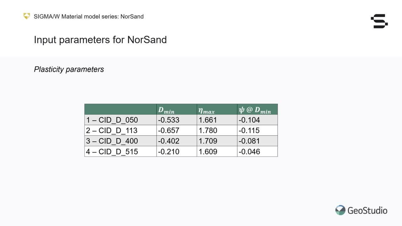
For each drained triaxial compression test performed

[00:17:41.020]
on dense sand in the dataset,

[00:17:42.383]
we would want to identify these three important points,

[00:17:45.932]
the maximum dilation,

[00:17:47.458]
the stress ratio at maximum dilation,

[00:17:50.278]
and the state parameter at maximum dilation.

[00:17:54.040]
It is important that only dense samples are used

[00:17:56.730]
for this step

[00:17:57.630]
since there wouldn’t be any maximum dilation

[00:17:59.910]
to identify for a loose simple by definition.

[00:18:04.080]
For our dataset,

[00:18:04.992]
this process would yield the following values.

[00:18:08.914]
By plotting these together on two separate plots,

[00:18:12.863]
we can see trends emerging,

[00:18:14.920]
which will allow us to determine three

[00:18:17.620]
of NorSand’s input parameters.

[00:18:20.090]
On plot A,

[00:18:20.923]
which is the maximum stress ratio

[00:18:22.640]
as a function of maximum dilation,

[00:18:24.706]
the y-intercept corresponds to the critical state ratio Mtc.

[00:18:29.606]
The slope of this best fit line would then be related

[00:18:33.040]
to the value metric coupling coefficient, N.

[00:18:36.270]
On plot B,

[00:18:37.570]
which is the maximum dilation as a function

[00:18:39.238]
of the state parameter at maximum dilation,

[00:18:41.997]
the slope of the best fit would correspond

[00:18:45.100]
to the state dilatancy parameter chi tc.

[00:18:48.383]
Notice that both chi tc

[00:18:50.660]
and a critical state ratio Mtc have the tc subscript.

[00:18:55.299]
This indicates that these parameters are specific

[00:18:58.180]
to triaxial compression.

[00:18:59.629]
The corresponding internal model parameters vary

[00:19:02.900]
when loading conditions depart from triaxial compression.

[00:19:06.207]
Also note that the best fit line on plot B

[00:19:08.952]
should pass through the origin as by definition,

[00:19:12.150]
dilation should be zero

[00:19:14.060]
when the state parameter is zero.

[00:19:16.486]
Now that most of NorSand’s input parameters were defined,

[00:19:19.471]
we are only left with parameterizing

[00:19:21.459]
the elastic shear modulus at the reference pressure

[00:19:23.938]
and the base value of the plastic hardening modulus.

[00:19:27.056]
While the role of the elastic shear modulus is obvious,

[00:19:30.526]
it is less so for the hardening modulus.

[00:19:33.341]
The plastic hardening modulus, H controls the rate

[00:19:36.208]
of hardening of the yield surface.

[00:19:38.690]
H is built using two of NorSand’s input parameters,

[00:19:42.197]
a base value H zero

[00:19:44.756]
and a dependent value Hy which is optional

[00:19:47.645]
and used to impose a dependence on the state parameter.

[00:19:50.944]
We will see later on how this can be used

[00:19:53.540]
to generalize the model.

[00:19:54.762]
Notice that when Hy is equal to zero,

[00:19:58.367]
which is a default value, H is simply equal to H zero.

[00:20:02.964]
The hardening of the yield surface refers to a change

[00:20:05.682]
in the yield surface size in position.

[00:20:08.603]
Here is NorSand’s yield surface.

[00:20:11.310]
It erupts a similar teardrop shape

[00:20:13.210]
as the original Cam-Clay model.

[00:20:15.261]
The yield surface that emits the elastic

[00:20:17.320]
from the elasto-plastic region.

[00:20:19.148]
A stress point that is located inside the yield surface

[00:20:23.580]
will only produce elastic deformations upon loading.

[00:20:26.639]
A stress point located exactly

[00:20:28.930]
on the yield surface will produce both elastic

[00:20:31.800]
and plastic deformations.

[00:20:33.737]
And finally a stress point located

[00:20:35.750]
outside the yield surface is inadmissible.

[00:20:39.094]
To reach a stress point at sea,

[00:20:41.161]
the yield surface would have to expand,

[00:20:43.756]
a mechanism called hardening.

[00:20:46.241]
It is precisely this aspect of the model

[00:20:48.266]
that the plastic hardening modulus, H controls.

[00:20:51.562]
How much hardening occurs

[00:20:52.785]
for a given plastic shear strain increment

[00:20:55.730]
is determined by H’s value.

[00:20:58.235]
This parameter is calibrated

[00:20:59.754]
using a trial and error procedure

[00:21:02.010]
using NorSand’s simulation results.

[00:21:04.810]
Now that we have reviewed the input parameters required

[00:21:07.020]
to use NorSand,

[00:21:08.340]
we can move on to using the model and SIGMA/W

[00:21:11.460]
to complete the calibration procedure.

[00:21:13.790]
A good practice before jumping into SIGMA/W

[00:21:16.210]
to calibrate a model is to properly organize our test data.

[00:21:20.369]
This can easily be done using Microsoft Excel.

[00:21:23.569]
Here is how I like to set this up.

[00:21:28.280]
This workbook contains all the laboratory results

[00:21:30.573]
that I have available to adjust NorSand’s parameters

[00:21:33.106]
for the Fraser River sand.

[00:21:35.581]
I created a summary sheet where each test is identified.

[00:21:39.702]
I also identified the initial conditions related

[00:21:42.345]
to each test as I will need these values

[00:21:44.916]
to set up the SIGMA/W simulations.

[00:21:47.720]
Finally, the known input parameters

[00:21:49.730]
for NorSand previously determined also indicated.

[00:21:53.288]
This will be common to all the simulations.

[00:21:56.715]
The parameters identified in red are those that need

[00:21:59.685]
to be adjusted using the simulation results from SIGMA/W.

[00:22:03.862]
In this other sheet are the various plots

[00:22:07.630]
that helped me fit the NorSand parameters

[00:22:09.830]
that were already discussed earlier.

[00:22:12.038]
You will recognize some of these plots.

[00:22:14.911]
Finally, all the other sheets

[00:22:17.419]
contain the laboratory test data.

[00:22:20.040]
Each sheet corresponds to one single test

[00:22:22.200]
where a few plots help me visualize each test.

[00:22:26.232]
For a drained test,

[00:22:27.606]
I like to view the stress point plot, this trespass plot,

[00:22:30.711]
the volumetric deformations,

[00:22:33.170]
and the state parameter evolution.

[00:22:35.445]
For a non-drained test,

[00:22:36.802]
instead of the volumetric deformations,

[00:22:38.797]
I plot the pore water pressure.

[00:22:41.019]
Let us use the test identified as CID_D_113

[00:22:47.090]
to start the parameter adjustment procedure in SIGMA/W.

[00:22:50.483]
This test is a drained test on dense sand.

[00:22:54.810]
Since there are already many tutorials available

[00:22:58.320]
on Geoslope’s website

[00:22:59.650]
on how to set up a triaxial in SIGMA/W,

[00:23:02.918]
I will go through these steps swiftly.

[00:23:05.929]
Feel free to download one of such examples for our website

[00:23:09.320]
if you are unfamiliar with some of the steps featured

[00:23:11.643]
in this part of the webinar.

[00:23:14.034]
First, I set up the product geometry for a triaxial test.

[00:23:28.225]
I used a 2D axisymmetric geometry to take advantage

[00:23:32.342]
of the triaxial simple cylindrical shape.

[00:23:36.760]
This allows me to only model a quarter of the sample.

[00:24:17.388]
I then create the SIGMA/W low deformation analysis

[00:24:21.640]
to apply the stresses that exist

[00:24:23.270]
at the end of the consolidation phase.

[00:24:55.540]
I create the simple isotropic elastic material model here,

[00:24:59.400]
as the deformations are irrelevant for this step.

[00:25:03.290]
Our goal is simply to establish the proper stresses

[00:25:05.638]
that exist at the start of the triaxial test.

[00:25:22.820]
I apply boundary conditions

[00:25:24.098]
to represent the confining stresses

[00:25:26.117]
to which the real sample was subjected.

[00:25:57.340]
A single higher order element,

[00:25:59.230]
which reduce integration will surface given

[00:26:01.245]
that there are no special variability of stress and strain.

[00:26:05.910]
I can start the analysis and verify

[00:26:07.680]
that the stresses are correctly applied to the sample.

[00:26:43.034]
The next step is to create

[00:26:44.157]
a new SIGMA/W low deformation analysis

[00:26:47.108]
to perform the shearing phase of the triaxial test.

[00:27:06.645]
Tolerable errors and number of steps are adjusted

[00:27:09.810]
to produce better results when using NorSand.

[00:27:28.265]
A NorSand material model is created

[00:27:29.853]
and the parameters that are demanded

[00:27:31.980]
at the previous part of this webinar are entered.

[00:28:25.090]
Then a first try

[00:28:26.380]
for defining the four missing parameters is done.

[00:28:31.370]
We haven’t discussed the over consolidation ratio yet.

[00:28:34.486]
The overall consolidation ratio, OCRp is the ratio

[00:28:37.979]
of the current

[00:28:39.170]
over the historical maximum mean effective stresses.

[00:28:42.854]
The W input displays the subscript P to remind us

[00:28:46.565]
that the ratio is defined in terms of mean effective stress.

[00:28:50.790]
For sense, the OCR is normally never very high,

[00:28:54.096]
but it is generally correct

[00:28:55.837]
to assume that a little over consideration exist

[00:28:58.717]
in a triaxial sample.

[00:29:00.847]
A value of 1.1 is used here.

[00:29:04.390]
For sands, values between one and 1.3 are normally expected

[00:29:08.047]
and generally will not have an overly important impact

[00:29:11.570]
on the simulation results,

[00:29:12.756]
especially for drained simulations.

[00:29:17.010]
Next is the shear modulus at the reference pressure.

[00:29:20.190]
There are many ways to generate the first guess

[00:29:21.755]
of this value.

[00:29:23.220]
Use whichever method you prefer.

[00:29:25.730]
From my geo-technical engineering courses

[00:29:27.358]
back in university,

[00:29:28.486]
I have always remembered that Young’s modulus

[00:29:31.220]
for sense can be approximated using the relationship N,

[00:29:34.620]
the SPT low count times 2000.

[00:29:37.923]
Young’s modulus divided by two

[00:29:40.000]
times one plus Poisson’s ratio

[00:29:42.540]
will then yield the elastic shear modulus.

[00:29:45.787]
For a Poisson’s ratio roughly estimated to 0.25

[00:29:49.802]
to keep digits easy to work with,

[00:29:52.066]
this would mean that I could estimate the shear modulus, G

[00:29:55.690]
as being N, the SPT blow count times 800.

[00:29:59.435]
Let us estimate

[00:30:00.323]
that our somewhat dense could have an SPT blow count of 25,

[00:30:04.820]
which would yield an estimated shear modulus of 20,000 kPa.

[00:30:08.893]
While an N value of 25

[00:30:10.565]
would technically not be considered dense in the field,

[00:30:13.970]
it would probably correspond to a dense sample built

[00:30:16.940]
in the laboratory for a triaxial test.

[00:30:19.530]
This is of course just a roughest estimate to get us going.

[00:30:22.510]
I like this method because I can genuinely get this estimate

[00:30:25.507]
in my head just by remembering this simple relationship.

[00:30:30.319]
Next is the plastic hardening modulus, H.

[00:30:33.743]
As I said earlier,

[00:30:34.802]
it is good practice to first neglect the effect

[00:30:37.068]
of the state parameter psi on the hardening modulus

[00:30:39.883]
by setting Hy to zero.

[00:30:42.789]
We will come back to this value later,

[00:30:44.930]
but for now we assume that the hardening modulus

[00:30:47.316]
is simply equal to H zero.

[00:30:49.542]
The plastic hardening modulus value generally sits

[00:30:52.970]
between 20 to 400.

[00:30:55.063]
And a good first estimate for it is H is equal

[00:30:59.290]
to four divided by Lambda,

[00:31:01.188]
the slope of the critical state line.

[00:31:03.597]
In our case

[00:31:04.840]
since we use a curve critical state line,

[00:31:06.820]
Lambda is not defined.

[00:31:08.130]
So let us just use a value of 60 as a starting point.

[00:31:12.178]
Finally, let us consider S, the additional softening index.

[00:31:17.077]
This is a feature

[00:31:18.093]
which helps NorSand correctly simulate the response

[00:31:20.960]
of loose soils being loaded under undrained condition.

[00:31:24.302]
S can take values from zero to one,

[00:31:27.550]
but is generally used with either one or zero,

[00:31:30.508]
like an on-off switch if you will.

[00:31:33.254]
For any drained test, S should always be kept to zero.

[00:31:37.750]
For a non-drained test, if the sample is dense,

[00:31:40.800]
for example if the state parameter is smaller than zero,

[00:31:43.333]
then S should also be kept to zero.

[00:31:46.219]
However, if the sample is loose,

[00:31:48.301]
for example if the state parameter is larger than zero,

[00:31:51.132]
then S could be non-zero.

[00:31:53.775]
I will show the effect of S equal one

[00:31:56.720]
for some undrained examples later on.

[00:31:59.310]
For now, since the test we are calibrating is strain,

[00:32:02.070]
S will be set to zero.

[00:32:06.760]
Back to SIGMA/W, we can now input the missing parameters

[00:32:10.540]
we just discussed to complete our definition

[00:32:12.355]
of the NorSand material.

[00:32:29.550]
The last step remaining before solving this analysis

[00:32:31.744]
is to create the boundary conditions needed

[00:32:34.007]
to perform a triaxial compression test

[00:32:36.638]
meaning that the top part

[00:32:37.931]
of the sample be made to move downward.

[00:32:56.452]
By creating a dense displacement function,

[00:32:59.600]
I can ensure that the top nodes will move down

[00:33:01.760]
by 0.01 meter,

[00:33:04.070]
which corresponds to 20% of vertical deformation

[00:33:06.872]
for the size of our sample.

[00:33:27.670]
I can now go ahead and remove the stress boundary conditions

[00:33:30.470]
that were created for the stress initialization step

[00:33:32.707]
as we don’t need these anymore.

[00:33:36.320]
The parent analysis,

[00:33:37.240]
which this current analysis depends on,

[00:33:39.603]
will transfer it’s stress conditions to its child.

[00:33:44.630]
I now apply the newly created displacement boundary

[00:33:46.625]
condition to the top of the sample.

[00:33:50.040]
As a side note,

[00:33:51.400]
the function should be defined over an elapsed time

[00:33:53.744]
that is commensurate with the duration of the analysis.

[00:33:57.130]
For example a one day.

[00:33:58.581]
That way, the number of steps used

[00:34:01.310]
to simulate the total vertical straining can be varied

[00:34:04.290]
without having to change the boundary condition.

[00:34:07.082]
We are now ready to solve the analysis.

[00:34:20.450]
Once this is done,

[00:34:21.445]
I can create plots to view the data

[00:34:23.903]
and to export it to Excel

[00:34:25.720]
to compare the NorSand results with the laboratory data.

[00:34:28.655]
To do so, I can select all my plots,

[00:34:31.760]
which are conveniently expressed in terms of vertical strain

[00:34:34.347]
and right click on a plot to select copy graph data.

[00:34:38.960]
Once plotted alongside the laboratory results,

[00:34:41.671]
I can visually inspect the simulation results

[00:34:44.358]
and evaluate the model’s performance.

[00:34:46.867]
In this case,

[00:34:47.962]
it looks like the model stress strain curve on plot A,

[00:34:51.450]
the orange curve is too soft compared

[00:34:53.339]
to the laboratory results, the green curve.

[00:34:56.440]
It is however worth pointing out that this first estimate

[00:34:59.430]
already provides a very acceptable fit compared

[00:35:01.485]
to the laboratory data.

[00:35:03.433]
This showcases the benefits of being able to adjust most

[00:35:06.522]
of NorSand’s parameters straight from laboratory data.

[00:35:11.140]
By returning to Joules to do

[00:35:12.560]
and adjusting the indicated parameters,

[00:35:14.314]
I can obtain what we will call the best fit.

[00:35:17.610]
Judging that simulation results

[00:35:19.430]
represent the best fit possible

[00:35:20.724]
is of course quite subjective

[00:35:22.678]
and there might be various combinations of parameters

[00:35:25.680]
that will lead to similar fits.

[00:35:28.970]
Care must be taken to avoid using unrealistic values.

[00:35:32.690]
For example, one can hardly expect OCR

[00:35:34.487]
is larger than 1.5 for sands

[00:35:36.700]
or shear moduli larger than 200,000 kPa.

[00:35:41.358]
When I’m satisfied with the fit I obtained,

[00:35:43.273]
I want to leave a trace of the final parameters I use

[00:35:46.680]
for this specific test.

[00:35:48.377]
To do so, I will return to my Excel summary worksheet

[00:35:52.174]
and input the chosen parameters

[00:35:54.880]
under the test I was working on.

[00:35:57.450]
I will then proceed similarly

[00:35:58.600]
with all the tests I have in hand,

[00:36:00.900]
using the same steps I just described.

[00:36:02.712]
I will use the same geometry,

[00:36:05.431]
but we’ll add new stress initialization

[00:36:07.745]
and triaxial compression phases for each test.

[00:36:11.379]
The stress boundary conditions are specific to each test.

[00:36:20.967]
In addition, the NorSand material models

[00:36:24.048]
are defined uniquely for each test

[00:36:25.683]
representing the appropriate initial conditions indicated

[00:36:29.110]
in my Excel summary worksheet.

[00:36:31.424]
I will follow the same procedure where I make a first guess

[00:36:35.350]
of the missing material parameters

[00:36:36.688]
and proceed to adjust them until I reach a satisfying fit.

[00:36:41.170]
We will work on normalizing these first guess parameters

[00:36:44.320]
at a later stage of the procedure.

[00:36:47.700]
I will finally record the best fit parameters

[00:36:50.620]
for all the tests in my Excel summary workbook.

[00:36:53.840]
You will notice that for three of these tests,

[00:36:56.099]
the additional softening index was turned down.

[00:36:59.022]
This can be done since these tests respect the requirements

[00:37:01.955]
that they must have been performed

[00:37:04.050]
in non-drained conditions for loose soils.

[00:37:06.596]
Here’s an example of the effector

[00:37:08.611]
in the additional softening index can have on such tests.

[00:37:12.439]
These other simulation results we obtain

[00:37:14.732]
when we use the default S value,

[00:37:17.200]
which is zero

[00:37:18.420]
for a test where static liquefaction is observed.

[00:37:21.388]
We can see that the responses much differ

[00:37:23.956]
for NorSand than for the laboratory results.

[00:37:27.114]
In particular, notice on plot D how NorSand

[00:37:30.350]
is still very far from critical state

[00:37:32.510]
whereas that parameter plot will be zero

[00:37:34.471]
while the laboratory results

[00:37:36.290]
on the contrary fairly quickly reached critical state.

[00:37:39.720]
By simply turning the additional softening index on,

[00:37:42.937]
we can get these results instead.

[00:37:45.210]
NorSand is now able to capture every aspect

[00:37:48.320]
of the static liquefaction behavior very nicely

[00:37:50.773]
producing large pore water pressure

[00:37:53.610]
that drives the main stress to very low values,

[00:37:55.938]
generating large deformations for minimal stress increments.

[00:38:00.240]
Although the additional softening index should only be used

[00:38:03.280]
after thoughtful consideration,

[00:38:04.846]
it can greatly help

[00:38:06.300]
to properly simulate some more complex aspects

[00:38:08.742]
of loose soil behavior.

[00:38:11.099]
Back to our Excel summary worksheet,

[00:38:13.595]
now that we have defined the NorSand input parameters

[00:38:16.930]
for every laboratory test we had available,

[00:38:19.019]
we can explore the possibility of generalizing some

[00:38:21.506]
of the input parameters to obtain a set of parameters

[00:38:25.060]
that would be as consistent as possible

[00:38:27.370]
across all the tests studied.

[00:38:29.424]
This should be done

[00:38:30.650]
in order to render our NorSand material more flexible.

[00:38:33.707]
In an ideal situation,

[00:38:35.370]
all the input parameters should remain the same,

[00:38:38.560]
no matter what the test conditions we encounter are.

[00:38:42.104]
Let us focus on the elastic shear

[00:38:44.830]
and plastic hardening moduli,

[00:38:46.412]
and how these two input parameters seem

[00:38:48.960]
to depend on the initial state parameter.

[00:38:51.357]
This would help us generalize our inputs

[00:38:53.584]
to make NorSand easier to use in real life simulations.

[00:38:57.808]
I have plotted the plastic hardening modulus on the left

[00:39:00.930]
and the elastic shear modulus at the reference pressure

[00:39:04.080]
on the right,

[00:39:05.030]
both as a function of the initial state parameter.

[00:39:07.698]
These plotted values are the best fit parameters

[00:39:10.380]
I have adjusted using SIGMA/W.

[00:39:13.210]
As it can be expected,

[00:39:14.043]
both moduli show a dependency

[00:39:16.620]
on the initial state parameter.

[00:39:18.227]
For both, denser soils will yield larger moduli.

[00:39:23.010]
By passing a linear regression line through both series

[00:39:26.380]
of data, I can define simple relationships

[00:39:28.534]
which can help automatically choose moduli values

[00:39:31.680]
that will yield good simulation results

[00:39:33.572]
no matter the initial conditions.

[00:39:36.394]
Specifically for the plastic hardening modulus H,

[00:39:39.615]
the two parameters of the linear regression curve

[00:39:42.500]
can be used directly in SIGMA/W as input values

[00:39:45.287]
that will directly take

[00:39:46.790]
into account the initial state of the soil.

[00:39:49.544]
The next version of SIGMA/W

[00:39:51.420]
to be released during the spring of 2021

[00:39:53.380]
will also feature similar state dependent capabilities

[00:39:56.465]
for the elastic shear modulus.

[00:39:59.614]
Let us take a final look at the Excel summary worksheet.

[00:40:04.202]
Now that I have defined state dependent relationships

[00:40:06.917]
for both moduli,

[00:40:08.572]
I can begin the chosen H zero and Hy values.

[00:40:12.947]
I can then use the elastic shear modulus relationship

[00:40:16.000]
to calculate the generalized shear modulus

[00:40:18.053]
at reference pressure for each test.

[00:40:21.400]
This allows me to finally define a complete NorSand model

[00:40:24.480]
that is almost entirely dependent

[00:40:26.240]
on the initial state for its initial parameters.

[00:40:29.312]
A case could very well be made to also adopt a single value

[00:40:33.456]
of OCR for all the tests, say 1.15 for example.

[00:40:38.836]
The only parameter that would then be needed to be adjusted

[00:40:41.818]
by the user would be the additional softening index S

[00:40:46.290]
that still needs to be turned on manually

[00:40:48.069]
for undrained loading of loose soils.

[00:40:51.030]
Other than these caveats,

[00:40:52.876]
the NorSand model we established

[00:40:54.565]
provides all the necessary parameters

[00:40:56.681]
to properly simulate the behavior

[00:40:58.910]
of the Fraser River sand for triaxial loadings

[00:41:01.730]
that include dense as well as loose initial states

[00:41:04.419]
and undrained as well as drained conditions.

[00:41:09.322]
To showcase the power of the procedure we just completed,

[00:41:12.253]
let us compare simulation results

[00:41:14.270]
for the best fit possible against the final fit,

[00:41:17.256]
using the generalized expressions for the elastic shear

[00:41:20.570]
and plastic hardening moduli for a few tests.

[00:41:24.330]
These are the simulation results

[00:41:26.440]
for a drained triaxial test performed on dense sand.

[00:41:29.472]
The green curves are the lab results

[00:41:31.314]
and the red curves are the NorSand simulations

[00:41:34.200]
for SIGMA/W with parameters chosen

[00:41:36.670]
to produce the best fit possible.

[00:41:39.188]
Finally, the dashed blue curves are the SIGMA/W results

[00:41:43.350]
using the input relationships developed

[00:41:45.068]
in the preceding steps that use the initial state parameter

[00:41:49.220]
to initiate the shear and hardening moduli.

[00:41:52.310]
The two NorSand simulation sets

[00:41:53.940]
are very close to each other.

[00:41:55.430]
And overall, very close to the laboratory results.

[00:41:58.746]
Even when using the input relationships,

[00:42:01.285]
NorSand clearly captures the soil behavior.

[00:42:03.847]
As expected, the dense soil shows some initial contraction

[00:42:08.470]
followed by important dilation

[00:42:10.450]
that will bring the soil closer

[00:42:11.830]
to its critical state at large deformation.

[00:42:15.067]
Here’s an undrained test performed on loose sand

[00:42:18.447]
where as another test showed earlier,

[00:42:21.036]
static liquefaction is involved.

[00:42:23.749]
Again, the NorSand simulation

[00:42:26.110]
using the state dependent input relationship are very close

[00:42:29.200]
to the best fit possible.

[00:42:31.546]
Very contractive behavior is observed

[00:42:34.036]
and the soil is quickly reaching its critical state.

[00:42:37.641]
Both simulations closely follow

[00:42:39.533]
the laboratory result behavior

[00:42:41.589]
and correctly stimulate static liquefaction.

[00:42:44.560]
This is a really great example of the strength of NorSand.

[00:42:48.750]
With a constant set of input parameters

[00:42:50.310]
coupled with state dependent relationships,

[00:42:52.330]
one can simulate dilatant

[00:42:55.290]
as well as very contracted behaviors.

[00:42:58.938]
As a last example,

[00:42:59.980]
here are the simulation results

[00:43:02.320]
for a non-drained loading on dense sand.

[00:43:04.648]
Again, the SIGMA/W simulation results

[00:43:07.404]
using the state dependent relationships are very close

[00:43:10.750]
to the best fit possible.

[00:43:12.295]
Both simulations correctly follow the laboratory results

[00:43:15.586]
where an initial contraction phase accompanied

[00:43:18.414]
by a positive pore water pressure generation is followed

[00:43:22.582]
by a dilatant phase

[00:43:23.806]
during which negative pore water pressure are generated.

[00:43:29.147]
That concludes this webinar part

[00:43:30.710]
of the SIGMA/W material model series.

[00:43:33.560]
Three main topics were covered during this presentation.

[00:43:38.560]
At first, an introduction to NorSand was presented

[00:43:40.827]
where the basics of the soil model were discussed.

[00:43:43.996]
The various input parameters needed

[00:43:46.450]
to use NorSand in SIGMA/W were examined

[00:43:48.636]
with a special focus on how most

[00:43:51.220]
of them can be adjusted

[00:43:52.560]
using triaxial yield compression results directly

[00:43:55.570]
while some others need simulation results

[00:43:57.730]
from SIGMA/W to be properly defined.

[00:44:00.779]
Finally, we considered how to use NorSand and SIGMA/W.

[00:44:04.971]
Toward the end of the presentation,

[00:44:07.730]
a special focus was put

[00:44:08.604]
on how to generalize NorSand’s input parameters

[00:44:11.547]
to create a complete and flexible state dependent model,

[00:44:15.378]
which represents one of NorSand’s strength.

[00:44:18.497]
Our team of development engineers is already hard at work

[00:44:21.420]
to provide new improvements to NorSand in the next version

[00:44:24.693]
of SIGMA/W that should be released this spring.

[00:44:28.362]
Users will notably be able to define the shear modulus

[00:44:32.030]
at reference pressure as a function of void ratio.

[00:44:34.759]
It will also become possible to use the state parameter

[00:44:38.360]
as an input instead of the void ratio.

[00:44:41.803]
If you’d like some new features and capabilities added

[00:44:45.210]
to NorSand and SIGMA/W,

[00:44:46.798]
don’t hesitate to make suggestions

[00:44:48.274]
by submitting support requests.

[00:44:50.792]
We have now reached the end of this webinar.

[00:44:53.985]
A recording of the presentation will be available

[00:44:56.902]
to view online.

[00:44:58.768]
Please take the time to complete the short survey

[00:45:01.470]
that appears on your screen so that we know what types

[00:45:03.514]
of webinars you’re interested in attending in the future.

[00:45:07.506]
Thank you very much for joining us

[00:45:09.151]
and have a great rest of your day.

[00:45:11.480]
Goodbye.