SIGMA/W Material Model Series: Modified Cam Clay

This webinar will review this material model in SIGMA/W.

The Modified Cam Clay material model in SIGMA/W can be used to simulate clays and other soils that exhibit yielding and non-linear elastic-plastic deformation patterns. This webinar will introduce you to MCC model theory and formulation and step you through the analysis and calibration of a triaxial test in SIGMA/W. A comparison of laboratory data to the SIGMA/W results will also be presented.

Overview

Video Transcript

[00:00:06.900]
<v Kathryn>Hello, and welcome to this GeoStudio</v>

[00:00:08.510]
Material Model webinars series on Modified Cam Clay.

[00:00:12.810]
My name is Kathryn Dompierre,

[00:00:14.300]
and I’m a Research and Development Engineer

[00:00:16.300]
with the GEOSLOPE engineering team here at Seequent.

[00:00:19.860]
Today’s webinar will be approximately 30 minutes long

[00:00:23.340]
attendees can ask questions using the chat feature.

[00:00:26.290]
I will respond to these questions via email

[00:00:28.600]
as quickly as possible.

[00:00:30.520]
A recording of the webinar will be available

[00:00:32.530]
so participants can review the demonstration

[00:00:35.120]
at a later time.

[00:00:39.565]
GeoStudio is a software package developed for geotechnical

[00:00:42.600]
engineers and earth scientists comprise of several products.

[00:00:47.210]
The range of products allows users to solve

[00:00:49.490]
a wide array of problems

[00:00:50.700]
that may be encountered in these fields.

[00:00:54.440]
Today’s webinar will focus on SIGMA/W.

[00:00:58.040]
Those looking to learn more about the products,

[00:01:00.000]
including background theory,

[00:01:01.500]
available features and typical modeling scenarios

[00:01:04.440]
can find an extensive library of resources

[00:01:06.690]
on the GEOSLOPE website.

[00:01:09.290]
Here, you can find tutorial videos,

[00:01:11.290]
examples with detailed explanations

[00:01:13.940]
and engineering books on each product.

[00:01:18.700]
To begin this webinar,

[00:01:19.660]
let us consider a soil element

[00:01:21.550]
using both the experimental approach

[00:01:24.350]
and a numerical approach.

[00:01:27.720]
And in experimental approach there’s a real soil sample

[00:01:30.590]
that is used for example, to conduct attracts yield test.

[00:01:34.770]
The responses of this soil sample are measured

[00:01:37.130]
in the laboratory and the soil behavior

[00:01:39.070]
can be studied accordingly.

[00:01:41.960]
And the numerical approach on the other hand,

[00:01:43.770]
it is necessary to perform a calibration process

[00:01:46.490]
for the constituent of model

[00:01:47.890]
as the first step of numerical modeling,

[00:01:51.430]
the measured results from the soil sample

[00:01:53.300]
are required at this step.

[00:01:56.720]
This calibration procedure provides model constants

[00:01:59.500]
for the soil.

[00:02:01.960]
These constants are then used as input parameters

[00:02:04.730]
for a numerical model

[00:02:06.230]
for example in SIGMA/W

[00:02:08.420]
and this simulated results will be obtained

[00:02:10.650]
by solving the numerical model.

[00:02:14.290]
The simulated results can then be compared

[00:02:16.450]
to the corresponding laboratory results

[00:02:18.920]
to verify the accuracy of the numerical modeling.

[00:02:23.040]
In today’s webinar the calibration procedure

[00:02:25.170]
for the modified Cam Clay material model will be provided.

[00:02:29.310]
This process will be applied to a specific type of Clay

[00:02:32.480]
as an example and the numerical values

[00:02:34.630]
of the model constants will be calculated.

[00:02:38.400]
The main steps of modeling attracts yield test

[00:02:40.670]
in SIGMA/W will be reviewed,

[00:02:43.810]
and the simulation results will be compared

[00:02:45.750]
to the experimental and analytical results

[00:02:48.170]
for validation purposes.

[00:02:52.010]
This webinar will begin by reviewing the theory

[00:02:54.370]
of the modified Cam Clay constituent of model.

[00:02:57.660]
Then step-by-step instructions will be provided

[00:03:00.160]
for calibrating this material model

[00:03:01.820]
using attracts field data series.

[00:03:05.350]
A demonstration of the steps of modeling attracts

[00:03:07.900]
yield test and SIGMA/W will be provided.

[00:03:10.500]
And the simulated results will become paired and verified

[00:03:13.240]
using the analytical and laboratory results.

[00:03:18.050]
The modified Cam Clay material model is a critical state

[00:03:21.030]
based non-linear constituent model

[00:03:23.430]
developed by Roscoe and Berlin in 1968.

[00:03:27.580]
In this model the author is modified

[00:03:29.300]
their previous constituent of model

[00:03:31.200]
by changing the geometry of the yield surface

[00:03:33.610]
from a bullet shape service to an ellipse.

[00:03:37.350]
For an isotropic loading condition

[00:03:39.420]
where the stress path is entirely located

[00:03:41.700]
on the horizontal axis.

[00:03:43.790]
The plastic strain increment vector is also horizontal

[00:03:48.010]
note that the plastic strain increment vector

[00:03:50.210]
is perpendicular to the yield surface.

[00:03:53.680]
The soil state is over consolidated

[00:03:55.730]
before reaching the yield surface.

[00:03:58.170]
After that the elliptical surface will be scaled up

[00:04:00.950]
as loading progresses.

[00:04:03.520]
The soil undergoes normal consolidation in this phase.

[00:04:08.870]
The soil response is assumed to be linear

[00:04:11.110]
in V versus lawn P prime space.

[00:04:14.620]
The slope of the normal consolidation line

[00:04:16.610]
is called the Virgin compression index or lambda

[00:04:20.490]
while the over consolidation and unloading, reloading lines

[00:04:23.610]
are assumed to be parallel.

[00:04:26.340]
Their slope is called the swelling index or Kappa.

[00:04:32.350]
In a deviatoric loading condition

[00:04:34.320]
where the vertical principles stress

[00:04:35.880]
is different than the horizontal one.

[00:04:38.090]
The stress path reaches the elliptical yield surface

[00:04:40.820]
at a point away from the horizontal axis.

[00:04:44.020]
This means that the plastic strain increment vector

[00:04:46.520]
contains deviatoric components as well.

[00:04:50.250]
In V versus lawn P prime space

[00:04:52.810]
the over consolidation and unloading, reloading phases

[00:04:56.100]
are still aligned with a slope of kappa.

[00:04:59.240]
However, the normal consolidation phase

[00:05:01.330]
is not necessarily a straight line

[00:05:03.370]
for a general and isotropic loading condition.

[00:05:08.980]
Before moving on to the demonstration,

[00:05:11.010]
we need to review some fundamental formulations.

[00:05:14.900]
As mentioned before the modified Cam Clay material model

[00:05:17.790]
is a critical state based constituent of model.

[00:05:20.460]
So different stress paths

[00:05:22.170]
eventually tend to the critical state line.

[00:05:25.650]
In this model the slope of the critical state line

[00:05:28.950]
or the critical state stress ratio

[00:05:31.400]
can be expressed in terms of the effective friction angle

[00:05:34.130]
in the more coolum failure criteria.

[00:05:38.590]
The yield surface is an ellipse

[00:05:40.360]
that passes through the origin

[00:05:42.060]
and intersects the critical state line

[00:05:44.120]
at its peak point.

[00:05:48.220]
The over consolidation ratio

[00:05:50.050]
is the ratio between the maximum isotropic stress

[00:05:52.840]
experienced by the soil

[00:05:54.280]
and the current isotropic stress of the soil.

[00:05:59.930]
For a stress state inside the yield surface

[00:06:02.300]
the soil response is elastic.

[00:06:04.440]
The compliance matrix is diagonal

[00:06:07.090]
and the bulk and shear modular are both proportional

[00:06:09.730]
to the mean effect of stress, P prime

[00:06:13.000]
and the specific volume V.

[00:06:17.520]
After reaching the yield surface and as it expands,

[00:06:20.640]
the soil response becomes elasto plastic

[00:06:23.630]
and non diagonal coupled components

[00:06:25.710]
appear in the compliance matrix.

[00:06:28.480]
Incremental strains in this condition

[00:06:30.450]
are the summation of elastic and plastic strains.

[00:06:33.530]
And so the current stress ratio plays a key role

[00:06:36.240]
in the soil response.

[00:06:40.690]
According to the framework proposed in the modified

[00:06:42.910]
Cam Clay model, the model constants include

[00:06:46.600]
the slope of the normal isotropic consolidation line

[00:06:49.280]
represented by lambda,

[00:06:51.670]
the slope of the over consolidation line or kappa,

[00:06:55.890]
the effective poisson’s ratio, new prime

[00:07:00.260]
and the effect of critical state friction angle, five-prime.

[00:07:04.700]
These four constants determined the soil type

[00:07:06.940]
based on the modified Cam Clay model.

[00:07:10.100]
Some other parameters will also be needed

[00:07:11.910]
to describe the initial conditions

[00:07:13.640]
of a specific soil sample.

[00:07:16.110]
These include the initial void ratio, the unit weight

[00:07:20.820]
and the over consolidation ratio.

[00:07:26.480]
In order to find the model constant

[00:07:28.140]
corresponding to a specific soil,

[00:07:30.410]
a step-by-step calibration procedure is discussed here

[00:07:33.370]
based on drain tracks, yield test results.

[00:07:36.800]
As the first step, the critical state stress ratio

[00:07:40.350]
M sub C or its equivalent,

[00:07:43.130]
the effect of critical state friction angle

[00:07:45.840]
can be estimated from drain tracks, yield test results.

[00:07:51.090]
According to critical state soil mechanics,

[00:07:53.240]
stress paths of samples

[00:07:54.550]
with different initial confining stresses

[00:07:56.950]
eventually tend to the critical state line

[00:07:59.000]
at their failure point.

[00:08:00.940]
Therefore, the critical state line

[00:08:02.480]
is a straight line that passes through the failure points.

[00:08:06.130]
The critical state stress ratio MC

[00:08:09.270]
is the slope of this line.

[00:08:12.600]
This constant can be calculated

[00:08:14.220]
using the method of least squares.

[00:08:18.300]
Since the failure criteria in the modified Cam Clay model

[00:08:21.210]
is the same as the more cooler model,

[00:08:23.200]
the effect of critical state friction angle five-prime

[00:08:26.190]
is not independent of the critical state stress ratio, MC

[00:08:30.720]
and can be expressed directly in terms of it.

[00:08:37.290]
To demonstrate the calibration procedure

[00:08:39.570]
let us consider three drained tracks yield compression tests

[00:08:43.040]
on Bothkennar clay that was conducted by McGinty in 2006.

[00:08:48.440]
These three tests have been performed

[00:08:50.010]
at different confining pressures.

[00:08:52.490]
The deviator compression stress

[00:08:54.240]
and these tests continued until failure was achieved.

[00:08:58.630]
The critical state line

[00:08:59.780]
that passes through the failure points

[00:09:01.610]
in P prime versus Q space has a slope of 1.36.

[00:09:07.750]
Thus, the critical state ratio MC is 1.36

[00:09:12.150]
and consequently, the effective friction angle

[00:09:14.390]
is calculated to be 33.7 degrees.

[00:09:21.480]
The second step of the calibration procedure

[00:09:23.600]
is to estimate the slope

[00:09:24.790]
of the over consolidation line or kappa.

[00:09:28.530]
For an over consolidated soil

[00:09:30.290]
kappa is the slope of the over consolidation line

[00:09:32.720]
and represents the elastic response of the sample.

[00:09:36.600]
The trends of the measured values of P prime and V

[00:09:39.230]
in this branch of the graph

[00:09:40.530]
can be projected to a straight line.

[00:09:43.280]
The slope of the Y intercept of this line

[00:09:45.400]
can be calculated directly

[00:09:46.910]
using the method of least squares.

[00:09:51.500]
An alternative method for estimating kappa

[00:09:54.160]
is to use the corresponding parameters

[00:09:56.210]
measured during an unloading, reloading process.

[00:09:59.540]
For a normally consolidated soil

[00:10:01.670]
the unloading reloading process

[00:10:03.280]
is required for estimating kappa.

[00:10:06.190]
The method of least squares can again be used

[00:10:08.220]
to calculate the slope and the Y intercept

[00:10:10.790]
of this straight line.

[00:10:15.660]
Let us apply the second calibration step

[00:10:17.680]
to the example, tracks yield test results

[00:10:20.010]
on Bothkennar clay mentioned earlier.

[00:10:23.380]
The over consolidation branch in each of these three curves

[00:10:26.550]
is projected to a straight line.

[00:10:29.700]
The slope of these three lines is almost the same

[00:10:32.650]
So their average 0.084 is used as the constant kappa

[00:10:37.890]
for this type of clay.

[00:10:43.110]
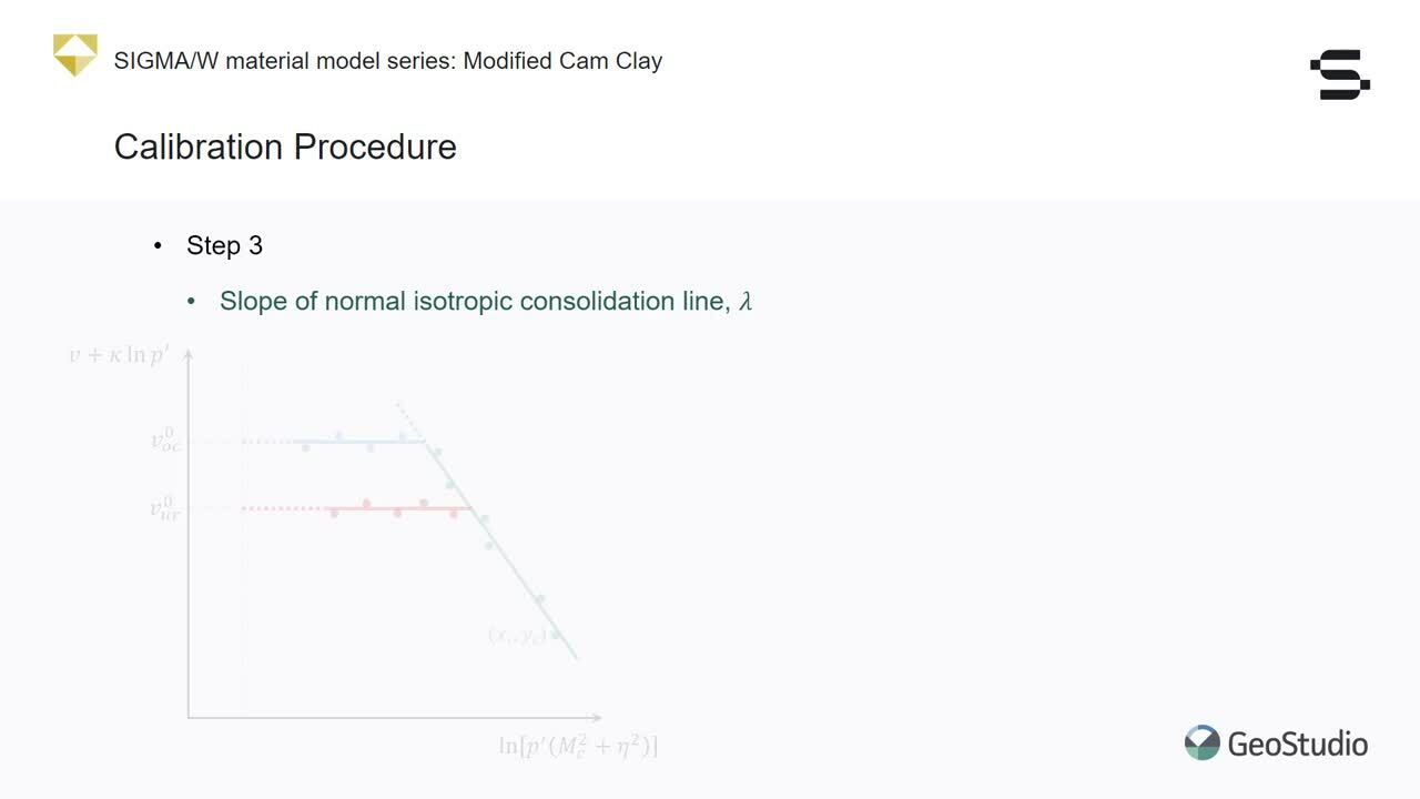
In the third step of the calibration procedure,

[00:10:45.980]
the slope of the normal isotropic consolidation line

[00:10:49.190]
or lambda will be estimated.

[00:10:51.990]
It should be noted that lambda’s the slope

[00:10:53.770]
of the normal consolidation line

[00:10:55.370]
only in an isotropic loading condition.

[00:10:58.520]
For other loading conditions however,

[00:11:00.320]
the normal consolidation branch

[00:11:02.340]
in V versus lawn P prime space is not necessarily linear.

[00:11:07.110]
And so the slope of its curve is obviously

[00:11:09.370]
not equal to lambda.

[00:11:12.630]
Based on the modified Cam Clay framework

[00:11:14.800]
it can be proved that there is an alternative space

[00:11:17.580]
in which the sample response is linear,

[00:11:19.580]
even under normal consolidation.

[00:11:22.110]
The X and Y axes in this space

[00:11:24.080]
are functions of the measured parameters

[00:11:26.040]
and constants estimated in the previous steps.

[00:11:30.640]
The over consolidation and unloading, reloading branches

[00:11:33.660]
are both horizontal in this new space.

[00:11:37.270]
And the normal consolidation branch

[00:11:39.470]
is a straight to sending line.

[00:11:42.390]
The slope of this line represents the difference

[00:11:44.410]
between the isotropic normal consolidation slope, lambda,

[00:11:47.900]
and the over consolidation slope, kappa.

[00:11:52.010]
Given that we already estimated kappa in the previous step,

[00:11:55.400]
the constant lambda can be found by applying

[00:11:57.710]
the method of least squares on the proposed space.

[00:12:04.650]
As shown in this figure,

[00:12:05.720]
the data points corresponding

[00:12:07.220]
to three example tracks yield test

[00:12:09.400]
are plotted in this alternate space.

[00:12:12.470]
The average value of the slopes of these three curves

[00:12:15.270]
in the normal consolidation branch

[00:12:17.080]
indicates the difference between lambda and kappa.

[00:12:20.960]
Since the value of kappa was previously obtained as 0.084

[00:12:25.960]
the constant lambda is estimated here to be 0.332.

[00:12:35.330]
The fourth step of the calibration procedure

[00:12:37.480]
is to calculate the over consolidation ratio

[00:12:39.870]
for each soil sample.

[00:12:42.640]
To do this, it is required to recognize

[00:12:44.960]
the mean effective pressure

[00:12:46.450]
in which the response of the sample changes

[00:12:49.070]
from the over consolidation condition

[00:12:51.170]
to the normal consolidation condition.

[00:12:55.250]
Let us refer to this pressure as the yield pressure

[00:12:57.890]
or P prime Y.

[00:13:00.880]
The over consolidation ratio however,

[00:13:02.790]
is the ratio between the isotropic

[00:13:05.200]
pre consolidation pressure P prime C,

[00:13:08.420]
and the isotropic initial pressure P prime zero.

[00:13:12.730]
As stated earlier the response of the soil changes

[00:13:15.410]
from an elastic or over consolidated state

[00:13:18.580]
to a elasto plastic or normally consolidated state

[00:13:22.090]
only if its stress path touches the yield surface.

[00:13:26.830]
As a result for a stress path that is not

[00:13:29.170]
necessarily isotropic the yield pressure P prime Y

[00:13:33.040]
is less than the isotropic

[00:13:34.600]
pre consolidation pressure P prime C

[00:13:38.240]
these two pressures however, are not independent.

[00:13:43.250]
For example, in a drain tracks yield stress pass

[00:13:45.810]
with a slope of three to one.

[00:13:47.830]
The deviatoric stress at the yield surface is three times

[00:13:50.980]
the difference between the yield and initial pressures.

[00:13:54.570]
So the isotropic pre-consultation pressure P prime C

[00:13:58.563]
can be expressed in terms of yield stresses

[00:14:00.757]
using the yield function of the elliptical surface.

[00:14:05.155]
Finally, the over consolidation ratio

[00:14:07.332]
is estimated as a ratio between

[00:14:09.254]
the isotropic pre consolidation pressure, P prime C,

[00:14:12.980]
and the isotropic initial pressure B prime zero.

[00:14:20.400]
This approach is applied on the Bothkennar clay

[00:14:22.550]
triaxial test data to estimate the over consolidation ratio

[00:14:26.520]
for each of the three samples.

[00:14:29.350]
First of all,

[00:14:30.183]
the yield points of the samples

[00:14:31.580]
in V versus lawn P prime space are detected.

[00:14:35.560]
The values of P prime Y for tests A1, A2 and A3

[00:14:41.090]
are about 83, 107 and 179 KPA respectively.

[00:14:47.630]
According to these yield pressures,

[00:14:49.310]
three yield surfaces are drawn

[00:14:51.060]
and the isotropic pre-consultation pressures

[00:14:53.590]
for three samples have been estimated as 115,

[00:14:58.680]
120 and 201 KPA respectively.

[00:15:04.220]
With this the over consolidation ratios for the samples

[00:15:07.440]
are found to be 2.069, 1.224 and 1.339.

[00:15:16.120]
Therefore the first sample is more over consolidated

[00:15:19.090]
than the other two samples.

[00:15:21.170]
This can also be deduced from the response of the sample

[00:15:23.950]
in V versus lawn P prime space,

[00:15:26.530]
where it has a longer elastic branch than the other samples.

[00:15:31.900]
The last step of the calibration procedure

[00:15:34.140]
for the modified Cam Clay constituent of model

[00:15:36.730]
is to determine the effective Poisson’s ratio, new prime.

[00:15:41.680]
Poissons ratio is defined as the ratio

[00:15:43.930]
of the change in the elements radio strain

[00:15:46.700]
to the change in its axial strain in a drained test.

[00:15:51.030]
In the modified Cam Clay model,

[00:15:52.930]
the Poisson’s ratio is considered only for the elastic

[00:15:56.150]
or over consolidated condition

[00:15:58.250]
and its value is assumed to remain constant during loading.

[00:16:03.230]
Consequently in a drain tracks yield test,

[00:16:06.050]
the method of least squares can be applied

[00:16:08.090]
on the purely elastic or over consolidated part of the curve

[00:16:12.010]
in radial strain versus axial strain space

[00:16:15.280]
to estimate the value of the effective Poisson’s ratio.

[00:16:21.030]
Lets us supply this final step to the Bothkennar clay

[00:16:23.370]
tracks yield test data.

[00:16:26.030]
The yield points of the samples have already been detected

[00:16:28.840]
in the previous steps and are marked with an X

[00:16:31.580]
in these figures.

[00:16:34.230]
As can be seen from the figure on the right

[00:16:36.520]
the sample response in this space is almost linear

[00:16:39.640]
before reaching the yield surface

[00:16:41.720]
while nonlinear behavior begins after yielding.

[00:16:46.430]
If the linear response of all three samples

[00:16:48.570]
was approximated by only one straight line

[00:16:51.040]
passing through the origin,

[00:16:52.800]
the slope of that line would be approximately 0.353.

[00:16:57.860]
This value is an estimation of the effective Poisson’s ratio

[00:17:01.420]
of the Bothkennar clay.

[00:17:06.750]
The results of the calibration procedure

[00:17:08.570]
for the Bothkennar clay can be summarized as follows

[00:17:11.760]
four model constants have been estimated,

[00:17:14.170]
including the slope of the normal

[00:17:15.830]
isotropic consolidation line,

[00:17:18.030]
the slope of the over consolidation line,

[00:17:20.500]
the effective Poisson’s ratio

[00:17:22.090]
and the effective critical state friction angle.

[00:17:25.770]
In addition the sample specific parameters

[00:17:28.010]
for these three tests include initial void ratios,

[00:17:31.360]
which were measured directly in the lab

[00:17:33.820]
and over consolidation ratios,

[00:17:35.770]
which were estimated in the calibration procedure.

[00:17:39.940]
These constants and parameters will be inputted in SIGMA/W

[00:17:43.280]
using the modified Cam Clay material model.

[00:17:49.120]
Now that we’ve reviewed the step-by-step

[00:17:50.700]
calibration procedure for the modified

[00:17:52.530]
Cam Clay material model,

[00:17:54.230]
I will describe how two model attract seal test in SIGMA/W

[00:17:57.830]
and compare the numerical results

[00:17:59.630]
with the previously mentioned laboratory data.

[00:18:02.980]
The numerical model configuration is based on the geometry

[00:18:06.200]
and boundary conditions of the tracks yield test

[00:18:08.440]
conducted in the laboratory.

[00:18:10.970]
A typical track yield test sample has a cylindrical shape

[00:18:14.320]
with a diameter of five centimeters

[00:18:16.250]
and a height of 10 centimeters.

[00:18:18.830]
Due to the axisymmetry shape of this geometry

[00:18:21.280]
with respect to the central vertical axis,

[00:18:24.050]
we can use the 2D axisymmetry geometry type in SIGMA/W.

[00:18:28.930]
The geometry is also symmetric with respect

[00:18:31.270]
to the horizontal axis.

[00:18:33.260]
So I will only model the top half

[00:18:35.010]
of the tracks yield sample.

[00:18:37.940]
An eight node Single element model

[00:18:40.250]
is considered for the resulting rectangle.

[00:18:43.170]
The left and bottom sides of this model

[00:18:45.040]
are fixed in the X and Y directions respectively,

[00:18:48.320]
while loads are applied to the other two sides.

[00:18:53.180]
The next step for setting up our SIGMA/W analysis

[00:18:55.780]
is the material definition.

[00:18:59.420]
This step is performed in the defined materials dialogue.

[00:19:02.570]
The material model is set to modified Cam Clay.

[00:19:06.300]
The sample parameters including the initial void ratio

[00:19:09.040]
and over consolidation ratio

[00:19:11.100]
are entered as discussed earlier.

[00:19:13.710]
It should be noted that the effect of the soil self weight

[00:19:16.430]
can be removed by setting the unit weight to zero.

[00:19:19.720]
While the key note effect can be deactivated

[00:19:22.460]
by specifying Key note and C as one.

[00:19:27.370]
Lastly, the constitutive model constants are entered

[00:19:30.410]
based on the results from the calibration procedure

[00:19:32.800]
for both Cam Clay.

[00:19:36.720]
The simulated tracks yield models are then loaded

[00:19:39.300]
under first, the isotropic confining pressure

[00:19:43.340]
and secondly the deviatoric pressure,

[00:19:47.200]
thus there are two SIGMA/W analysis required

[00:19:49.740]
for each of the triaxial tests.

[00:19:52.800]
The confining pressure analysis acts as the parent

[00:19:55.800]
and its results are used as the initial data

[00:19:58.200]
for the displacement controlled deviatoric analysis.

[00:20:03.020]
These conditions are established

[00:20:04.380]
using the boundary condition

[00:20:05.540]
specified in the defined boundary conditions dialogue.

[00:20:08.800]
For example, in test A1 the constant normal stress

[00:20:12.270]
of 58 KPA is applied on both the right and top sides

[00:20:16.390]
of the model using a normal tan stress boundary type

[00:20:19.920]
for the confining pressure analysis.

[00:20:23.340]
In the deviatoric analysis,

[00:20:25.260]
a displacement type boundary condition

[00:20:27.110]
is applied to the top of the model.

[00:20:29.660]
A displacement of two centimeters that is equivalent

[00:20:33.250]
to 40% strain is applied linearly over time

[00:20:37.150]
using a splined data point function.

[00:20:41.790]
All the analysis are then solved in SIGMA/W

[00:20:45.150]
and the stress, strain, displacement

[00:20:47.510]
and other responses of the model

[00:20:49.330]
can be extracted and interpreted.

[00:20:57.710]
As shown here a 2D axisymmetry geometry

[00:21:00.540]
is used to set up the model domain.

[00:21:03.170]
In the 2D view only one quarter of the cross-section

[00:21:06.230]
running through the center of the tracks yield sample

[00:21:08.700]
is modeled given the symmetry of the domain.

[00:21:12.610]
In the analysis tree, there are three sets of analysis

[00:21:15.640]
each representing attracts yield test

[00:21:17.670]
conducted on the Bothkennar clay samples.

[00:21:20.730]
In each test the confining phase is the parent analysis

[00:21:24.620]
and the deviatoric phase

[00:21:26.320]
that use the results of the previous phase

[00:21:28.570]
is the child analysis.

[00:21:32.140]
The material properties for three soil samples

[00:21:34.440]
were obtained using the outlined calibration procedure.

[00:21:38.070]
The materials are specified

[00:21:39.480]
in the defined materials dialogue.

[00:21:43.750]
The same type of clay

[00:21:44.810]
was subjected to the tracks yield tests.

[00:21:47.900]
Therefore, the Constance of the modified Cam Clay model

[00:21:51.040]
are similar for each sample.

[00:21:53.300]
However, at the initial void ratio

[00:21:55.810]
and over consolidation ratio are not the same

[00:21:58.460]
for each sample

[00:21:59.520]
and so three different materials were defined.

[00:22:14.750]
And isotropic elastic material was used

[00:22:17.680]
during the first phase of the tracks yield simulations,

[00:22:20.410]
because the nonlinear stress strain response

[00:22:23.390]
is inconsequential to establishing the initial stresses.

[00:22:27.640]
The accumulated displacements and strains are reset

[00:22:30.640]
at the start of the loading phase of the simulation.

[00:22:34.030]
The three isotropic elastic materials defined here

[00:22:37.640]
are applied to the corresponding, confining analysis.

[00:22:43.250]
The defined modified Cam Clay materials

[00:22:45.860]
are applied during the deviatoric portion of the tracks

[00:22:48.730]
yield test simulations.

[00:23:00.500]
The boundary conditions representing the confining pressures

[00:23:03.340]
and deviatoric strain are specified

[00:23:05.800]
in defined boundary conditions.

[00:23:08.040]
Three constant confining pressures were created

[00:23:10.710]
for the three tracks yield tests

[00:23:13.010]
using the normal 10 stress boundary type.

[00:23:16.840]
These boundary conditions

[00:23:18.010]
are applied to the corresponding confining analysis.

[00:23:31.600]
The deviatoric strain boundary for the displacement

[00:23:34.170]
control loading phase of the tracks yield test

[00:23:37.000]
uses the force displacement boundary type

[00:23:39.880]
with a displacement function defined

[00:23:42.000]
such that displacement increases

[00:23:43.740]
over the deviatoric strain analysis

[00:23:45.830]
from zero to two centimeters.

[00:23:52.970]
Before solving an analysis

[00:23:54.460]
the final step is to review the finite element mesh.

[00:23:58.070]
In the draw mesh properties dialog

[00:24:00.500]
we see that the global element mesh size is 0.05 meters

[00:24:05.670]
thus, the model domain represents one element.

[00:24:10.700]
This analysis has already been solved

[00:24:12.890]
so I will move to the results view.

[00:24:17.690]
I will go to the first deviatoric analysis

[00:24:19.970]
to investigate the results.

[00:24:22.560]
In the draw graph dialog, I have created graphs

[00:24:25.040]
to illustrate the stress path, stress strain curve,

[00:24:29.300]
and void ratio versus mean effect of stress.

[00:24:34.490]
I can click through the different analysis

[00:24:36.580]
to view the results from each.

[00:24:43.020]
Let us now compare these results

[00:24:44.710]
with the analytical solution

[00:24:46.680]
and also with the corresponding laboratory data.

[00:24:56.480]
The different simulation results of test A1

[00:24:59.300]
are compared here with the corresponding laboratory results.

[00:25:03.240]
Discrete scatter points represent the laboratory results

[00:25:07.100]
and the continuous black lines

[00:25:08.890]
are the SIGMA/W simulation results.

[00:25:12.550]
Analytical results for the modified Cam Clay model

[00:25:15.420]
are also shown in these diagrams as orange dashed lines.

[00:25:20.810]
The full compatibility of the analytical

[00:25:22.920]
and numerical curves shows the reliability

[00:25:25.860]
of the implementation process

[00:25:27.550]
of this material model in SIGMA/W.

[00:25:30.960]
When comparing the laboratory results

[00:25:32.710]
with the constituent of model simulations,

[00:25:35.400]
some of the plots show a better fit than others.

[00:25:38.440]
For instance, a very good match

[00:25:40.210]
can be seen in the first curve

[00:25:42.230]
where the data in V versus lawn P prime space

[00:25:45.640]
is simulated by the modified Cam Clay model.

[00:25:49.450]
However, the results from test A1

[00:25:51.400]
in some of the other spaces

[00:25:53.410]
do not match as nicely as the first curve

[00:25:56.330]
because of the very nature of calibration.

[00:25:59.740]
The calibration procedure highlighted in this webinar

[00:26:02.480]
required multiple samples,

[00:26:04.420]
which each have varying degrees of disturbance.

[00:26:08.010]
For example, during the calibration process,

[00:26:10.880]
the best fit line that was used to determine MC

[00:26:14.140]
was below the A1 and A3 data points,

[00:26:17.610]
but near the A2 data point,

[00:26:19.730]
thus, the simulated deviatoric failure stress

[00:26:22.570]
was underestimated for the A1 sample.

[00:26:26.820]
Meanwhile, the simulated deviatoric failure stress

[00:26:29.660]
better correlates to the laboratory results from test A2

[00:26:34.910]
and underestimates the deviatoric failure stress

[00:26:37.610]
for test A3.

[00:26:39.360]
This demonstrates the nature of the calibration process.

[00:26:42.350]
However, as mentioned for the first test,

[00:26:44.830]
the analytical and numerical results show a perfect match

[00:26:48.100]
verifying that SIGMA/W accurately represents

[00:26:50.540]
the modified Cam Clay material model.

[00:26:55.390]
In this webinar,

[00:26:56.560]
the calibration procedure of the modified Cam Clay

[00:26:58.890]
material model was provided in five straightforward steps.

[00:27:03.740]
The results of the drain tracks yield test,

[00:27:06.030]
where the only laboratory data set required for calibration.

[00:27:10.670]
The identified material constants

[00:27:12.850]
were used in a SIGMA/W numerical model,

[00:27:15.830]
and the simulation results were found to compare favorably

[00:27:19.490]
with both the analytical solution

[00:27:21.340]
and corresponding laboratory results.

[00:27:27.690]
Here are other references discussed in this webinar.

[00:27:38.020]
We’ve now reached the end of the webinar.

[00:27:40.040]
A recording of this webinar will be available

[00:27:42.020]
to view online.

[00:27:43.730]
Please take the time to complete the short survey

[00:27:45.940]
that appears on your screen

[00:27:47.270]
so we know what types of webinars

[00:27:48.810]
you are interested in attending in the future.

[00:27:51.780]
Thank you very much for joining us

[00:27:53.390]
and have a great rest of your day, goodbye.