SIGMA/W Field Stresses

This webinar demonstrates a practical example using the Field Stresses feature in SIGMA/W, as well as some practical tips for simulating initial stress in the subsurface.

Establishing the initial stress in the subsurface is key to conducting stress-strain analyses that captures the behaviour of the physical system. The presence of high in situ stress, for example, can lead to rock bursts or significant deformations in mining and tunnel applications. High stresses environments are common in complex geological systems in which tectonics or other geological processes lead to over-stressed rock, or in geotechnical applications at great depths. This webinar reviews field stresses and how they are used, including a practical example in SIGMA/W and tips for avoiding potential pitfalls.

Overview

Video Transcript

[00:00:00.140]
<v Instructor>Hello and welcome</v>

[00:00:01.210]
to this GeoStudio webinar focusing

[00:00:03.360]
on field stresses, one of the recent additions

[00:00:06.020]
to our products.

[00:00:07.850]
I’m Vincent Castonguay, I work as a research

[00:00:10.130]
and development specialist with

[00:00:11.470]
the Geoslope engineering team here at Seequent.

[00:00:14.700]
Today’s webinar will be approximately 30 minutes long.

[00:00:18.200]
Attendees can ask questions using the chat feature.

[00:00:21.160]
I will respond to these questions via email

[00:00:23.670]
as quickly as possible.

[00:00:25.690]
A recording of the webinar will also be available

[00:00:27.910]
so participants can move you the demonstration at

[00:00:30.440]
a later time.

[00:00:33.470]
GeoStudio is as a software package developed

[00:00:35.470]
for geotechnical engineers and earth scientists comprise

[00:00:38.700]
of several products.

[00:00:40.340]
The range of products allow users to solve

[00:00:42.830]
a wider array problems that may be encountered

[00:00:45.110]
in these fields.

[00:00:46.690]
Today’s webinar relate specifically to SIGMA/W.

[00:00:51.070]
Those looking to learn more about

[00:00:52.650]
the products including background theory, available features

[00:00:56.220]
and typical modeling scenarios can find an extensive library

[00:00:59.990]
of resources on the Geoslope website.

[00:01:02.850]
There you can find tutorial videos, examples

[00:01:05.650]
with detailed explanations and engineering books

[00:01:08.600]
on each products.

[00:01:11.730]
Calculating in situ stresses that applied to a domain

[00:01:14.580]
is one of the most important steps

[00:01:16.340]
in any stress train numerical analysis.

[00:01:19.430]
Large-scale geological processes

[00:01:21.510]
such as tectonic plate movements,

[00:01:23.750]
can greatly influence field stresses at large depth.

[00:01:27.410]
SIGMA/W webinar now offers an in situ analysis type that

[00:01:30.720]
can help easily specify these stresses.

[00:01:34.630]
Today’s webinar now will be divided into two parts.

[00:01:37.740]
We will first review the basics

[00:01:39.290]
of field stresses before looking into how

[00:01:42.190]
to use SIGMA/W model these.

[00:01:45.260]
Interested users are encouraged to download

[00:01:47.820]
the underground tunnel excavation practical example

[00:01:50.610]
from our website.

[00:01:51.790]
Which includes both an explanatory PDF

[00:01:54.710]
and a GeoStudio file.

[00:01:57.990]
There are three methods one can use

[00:01:59.810]
to initialize in situ stresses in a SIGMA/W analysis.

[00:02:04.620]
By using the gravity activation method, gravity is applied

[00:02:07.990]
to create a vertical stress field using the unit weight

[00:02:11.500]
of the soils involved.

[00:02:13.460]
Poisson’s coefficient and the geometry of the domain

[00:02:16.560]
will then control how a resentful stresses develop

[00:02:19.340]
in response to the vertical stresses.

[00:02:23.340]
As for the gravity activation,

[00:02:25.180]
the K naught procedure uses gravity to initiate

[00:02:28.060]
a vertical stress field in the domain.

[00:02:30.890]
This time however, horizontal stresses are calculated

[00:02:34.300]
by enforcing a defined K naught value.

[00:02:37.830]
Users should consult a SIGMA/W manual

[00:02:40.950]
for more information about the K naught procedure

[00:02:43.460]
and to learn when this procedure should

[00:02:45.920]
and should not be used.

[00:02:49.140]
The last way to initialize stresses in SIGMA/W

[00:02:52.450]
is to proceed via a user specified stress field.

[00:02:57.000]
In this case, gravity will be ignored in favor of a set

[00:03:00.630]
of stress quantities and directions specified better user.

[00:03:05.500]
At large depth, tectonic forces

[00:03:08.070]
and other large scale geological processes

[00:03:11.100]
can greatly influence institutes stresses producing

[00:03:15.120]
what are called locked-in stresses.

[00:03:17.850]
These stresses exist within the rock mass and cannot

[00:03:20.840]
be calculated by simply considering the unit weight

[00:03:23.670]
of the rocks and soils above like we conventionally do

[00:03:27.240]
for shallow ground calculations.

[00:03:30.200]
Tools such as the world stress map exists to help engineers

[00:03:33.270]
and geoscientists estimate the magnitude and orientation

[00:03:36.500]
of these locked-in stresses,

[00:03:38.220]
at various locations around the globe.

[00:03:40.830]
Direct measurement of stresses using stress cells

[00:03:43.510]
are indirect methods such as evaluating breakout orientation

[00:03:47.330]
in a tunnel arrays, are also use for determining

[00:03:50.720]
the in situ stress conditions.

[00:03:53.160]
Such tools provide the necessary inputs to specify

[00:03:56.590]
its field stressors for a SIGMA/W analysis,

[00:03:59.610]
where such stress patterns are expected.

[00:04:03.630]
As we will see in greater details later

[00:04:05.820]
on in this webinar via practical example, field stresses

[00:04:09.557]
are specified in SIGMA/W through the defined dropdown menu.

[00:04:14.120]
When defining new field stresses,

[00:04:16.270]
the major principle stress sigma one,

[00:04:18.810]
the minor principal stress sigma three

[00:04:21.460]
and the out of plane stress sigma Z are specified.

[00:04:25.260]
In addition, the direction

[00:04:27.430]
of the major principles stress alpha must also be specified.

[00:04:32.550]
The orientation is taken as positive counter-clockwise

[00:04:35.710]
from the x-axis.

[00:04:38.350]
The stresses hence defined will be applied uniformly

[00:04:41.290]
to each element from the regions that are selected.

[00:04:46.890]
Let us look at a few simple application cases.

[00:04:50.650]
Imagine this squared represents that domain

[00:04:52.800]
to which field stresses are to be applied.

[00:04:56.303]
Isotropic stresses of 10,000 kPa are applied here.

[00:05:00.500]
With alpha the principal stress direction being zero.

[00:05:04.010]
As sigma one is oriented along the x-axis.

[00:05:08.840]
By choosing a non-zero value for alpha

[00:05:11.200]
for example, minus 35 degrees here

[00:05:14.690]
the orientation of the applied stresses is rotated.

[00:05:18.730]
Remembered that alpha is positive counter-clockwise.

[00:05:22.150]
Here, I have also specified varied values

[00:05:25.770]
for the tree stress components, creating

[00:05:28.320]
an anisotropic stress field.

[00:05:31.160]
Remember that when specifying these stresses

[00:05:34.200]
the largest stress should always be sigma one,

[00:05:37.430]
the major principles stress.

[00:05:40.060]
I will use this stress pattern in the example that follows.

[00:05:44.860]
Before we move on to the practical example, let us review

[00:05:48.090]
a few important considerations.

[00:05:51.470]
The field stresses defined will be uniformly applied

[00:05:54.320]
to the whole domain that is selected.

[00:05:57.890]
Gravity’s ignored when initializing in situ stresses using

[00:06:01.730]
the field stresses method as stresses I specified

[00:06:04.587]
by the user.

[00:06:07.230]
A proper analysis three sequence using field stresses

[00:06:10.700]
will generally start with the

[00:06:12.410]
in situ field stresses analysis, followed

[00:06:15.460]
by stress correction analysis.

[00:06:17.560]
And finally, the load-deformations analysis

[00:06:20.970]
that were desired from the start.

[00:06:23.500]
This could be an excavation for example.

[00:06:27.340]
The stress correction analysis ensures

[00:06:29.440]
that no stress state breaches

[00:06:31.480]
its yield criterion following

[00:06:33.160]
the stress initialization procedure.

[00:06:37.100]
Let us now consider a practical example

[00:06:39.510]
where field stresses are used in GeoStudio.

[00:06:44.510]
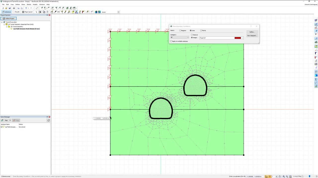
Here is the geometry we will be working with.

[00:06:47.600]
This represents two tunnels to be excavated at large depth.

[00:06:52.130]
I generated the geometry from a DWG drawing

[00:06:56.120]
that was imported into Build3D,

[00:06:58.520]
the companion software we use with our 3D products

[00:07:01.670]
and then export it back into GeoStudio.

[00:07:05.750]
Any other methods to create your model geometry

[00:07:08.530]
would also work here.

[00:07:10.830]
As described a moment ago, the first step for these types

[00:07:14.180]
of problems is to add an in situ analysis using

[00:07:18.040]
the field stresses method.

[00:07:20.420]
The first example is going to use

[00:07:22.640]
the Hoek-Brown material model, so let us identify this

[00:07:26.750]
in the analysis name.

[00:07:30.000]
We didn’t need to specify the pattern

[00:07:32.300]
of field stresses we want to apply to our domain.

[00:07:35.890]
We then need to specify the pattern

[00:07:37.600]
of field stresses we want to apply to our domain.

[00:07:40.800]
I will be using the pattern shown earlier

[00:07:43.140]
where the major principle stress sigma one is oriented

[00:07:46.440]
at an angle of minus 35 degrees from the x-axis,

[00:07:50.490]
with a value of 12,000 kPa.

[00:07:53.520]
The minor principles sigma three, takes a value

[00:07:56.740]
of 8,000 kPa.

[00:07:58.770]
And finally, the out of plane stress sigma Z, takes

[00:08:02.050]
a value of 10,000 kPa.

[00:08:04.800]
I can then draw this field stresses definition

[00:08:07.600]
onto my entire domain.

[00:08:10.920]
Let us now define the material we will be using

[00:08:13.370]
for this analysis.

[00:08:14.920]
I chose to hook brown material model to represent

[00:08:17.300]
a bedrock we are working with at depth.

[00:08:19.800]
This is obviously just an example.

[00:08:21.790]
Use whichever material model fits your specific needs.

[00:08:25.670]
I then apply this material to every region of my domain,

[00:08:29.220]
since I suppose the rock is very homogenous here.

[00:08:34.060]
The next step is to apply proper boundary conditions.

[00:08:37.550]
These are quite simple for such an analysis, as we will fix

[00:08:40.670]
the domain in both X and Y directions on each of its sites,

[00:08:44.900]
which is what is required for a field stresses analysis.

[00:08:54.650]
Lastly, make sure that secondary nodes are turned

[00:08:57.300]
on for better precision and that the size of

[00:08:59.830]
the elements is appropriate.

[00:09:09.840]
I can now run the analysis and let the solver apply

[00:09:12.347]
the field stresses to the domain.

[00:09:17.120]
Once the solver is done, I can verify that the stresses

[00:09:19.810]
are correctly applied by going into results

[00:09:22.600]
and then view result information.

[00:09:25.730]
I can set at any element in the domain

[00:09:27.470]
and verify that the maximum

[00:09:29.120]
and minimum total stresses correctly correspond to the major

[00:09:33.090]
and minor in principal stresses sigma one

[00:09:35.770]
and sigma three, I had specified earlier.

[00:09:39.260]
In this case 12,000 and 8,000 kPa respectively.

[00:09:43.760]
The out of plane stress sigma Z,

[00:09:45.770]
also correctly indicates 10,000 kPa.

[00:09:49.680]
Note here that since our principal stresses were defined at

[00:09:52.450]
an angle of 35 degrees, the maximum

[00:09:55.760]
and minimum stressors do not coincide with

[00:09:58.370]
the horizontal and vertical directions.

[00:10:00.990]
Causing the X and Y total stresses to take values in between

[00:10:04.680]
the major and minor principles stresses.

[00:10:08.290]
Finally, note that I could have chosen any element

[00:10:11.460]
in the domain since field stresses

[00:10:13.217]
are applied uniformly throughout the domain.

[00:10:17.740]
The next step once we verified our stresses

[00:10:20.007]
are correctly applied, is to perform

[00:10:21.900]
a stress correction analysis to ensure

[00:10:24.250]
that no stress point lies in illegal stress space.

[00:10:28.010]
Let us go back to define project

[00:10:30.010]
and add a stress to distribution analysis using

[00:10:32.810]
this stress correction method, that uses

[00:10:35.200]
the stresses defined in the previous step as inputs.

[00:10:40.700]
After I’ve solved this analysis I can view if there

[00:10:43.410]
were indeed some problematic stress points in my domain

[00:10:46.240]
by toggling view plastic states on the right side

[00:10:49.540]
of the screen.

[00:10:51.620]
In this case, all was good since there are no elements

[00:10:55.000]
that turned yellow.

[00:10:56.320]
In a separate example I will show in a few minutes, we

[00:10:59.160]
will see how that looks when stresses have been corrected.

[00:11:02.870]
Now that I know I have a correctly defined stress field I

[00:11:05.630]
can proceed with the excavation of the first tunnel,

[00:11:08.730]
by adding a load information analysis to my analysis tree.

[00:11:17.140]
I will make sure to take the reset displacement

[00:11:19.390]
and strains tick boxes here to ensure strains

[00:11:22.650]
that I’ve occurred in the previous analysis

[00:11:25.460]
are not carried forward.

[00:11:27.280]
To simulate the excavation I simply removed

[00:11:30.010]
the material model that was attributed to the interior

[00:11:32.530]
of the tunnel.

[00:11:38.780]
I can now launch the solver.

[00:11:41.970]
Once the results have computed I

[00:11:43.990]
can view various results like

[00:11:45.720]
the accumulated displacement field in the domain.

[00:11:49.070]
Here we can see that the bottom of the excavation

[00:11:51.860]
is bulging up.

[00:11:53.630]
By exaggerating the mesh deformation, we can see

[00:11:57.040]
this more clearly.

[00:11:59.070]
In a sense the large stresses that exists in the domains

[00:12:02.410]
are causing the tunnel to close in

[00:12:04.470]
on itself following the excavation.

[00:12:07.700]
If these deformations or yielding were judged

[00:12:11.080]
to be excessive, a bolting pattern might be proposed

[00:12:14.210]
to mitigate the situation.

[00:12:17.480]
To monitor the formations that occur inside

[00:12:19.550]
the tunnel following the excavation I can plot

[00:12:22.260]
the total displacement for a specific point at the bottom

[00:12:24.990]
of the excavation.

[00:12:26.680]
Here we can see that the bottom experienced an uplift

[00:12:29.730]
of 75 millimeters following the excavation.

[00:12:35.160]
Another interesting set of results to view is the patterns

[00:12:38.130]
of horizontal and vertical stresses that

[00:12:41.050]
are generated around the excavation.

[00:12:43.850]
These stresses started at the values we viewed earlier,

[00:12:47.280]
but varied following the excavation

[00:12:49.090]
as deformations occurred.

[00:12:51.800]
As we proceed with the excavation of the second tunnel,

[00:12:54.590]
these modified field stresses will certainly have an impact

[00:12:57.560]
on stresses and strains that are generated further on.

[00:13:01.800]
Lastly, by toggling on the view plastic states option I

[00:13:05.580]
can see that a large portion of the elements surrounding

[00:13:08.160]
the excavation reached a hook brown yield criterion we

[00:13:11.220]
had fixed, which explains the large deformations we see.

[00:13:15.240]
I cannot proceed with the excavation of the second tunnel

[00:13:17.900]
by adding a second load deformation analysis as a child

[00:13:21.110]
of the first excavation, as we will be using the stresses

[00:13:24.410]
from the previous steps as inputs.

[00:13:27.770]
This time, I want to leave the reset check boxes off

[00:13:31.220]
since I want to display

[00:13:32.470]
the accumulated deformations resulting

[00:13:34.480]
from both excavations.

[00:13:36.940]
Again to simulate the excavation, I simply removed

[00:13:40.390]
the soil model from inside of the tunnel geometry

[00:13:43.270]
and I launched the analysis.

[00:13:52.860]
As you can see, the excavation of the second tunnel modified

[00:13:56.510]
the field stresses again,

[00:13:57.890]
which caused additional deformations to propagate including

[00:14:01.070]
in the first excavated tunnel.

[00:14:03.540]
By going back and forth from the first to

[00:14:05.550]
the second excavation phases in the analysis tree, I can see

[00:14:09.550]
how vertical and horizontal stresses varied

[00:14:12.140]
as a result of the second excavation.

[00:14:15.410]
As you can expect, the second excavation caused

[00:14:18.860]
the region of plastic states to expand even further.

[00:14:22.950]
This caused deformations in excess of 110 millimeter

[00:14:26.570]
to develop at the base of the first tunnel.

[00:14:31.140]
Let us not consider a second example using

[00:14:33.350]
the same geometry, but with different materials.

[00:14:36.900]
Since this simulation steps I want to perform will be

[00:14:39.660]
the same as the previous analysis I can simply right-click

[00:14:42.620]
on the first analysis and then select add analysis

[00:14:45.730]
and then clone.

[00:14:46.910]
And choose to clone the whole analysis branch.

[00:14:49.860]
I then update the names of the newly created analysis

[00:14:53.650]
to keep my analysis tree well-organized.

[00:15:11.230]
I have already created two materials for

[00:15:13.020]
this analysis, both using

[00:15:14.920]
the Mohr-Coulomb hardening softening material model.

[00:15:18.340]
The first material is called Mohr-Coulomb and represents

[00:15:20.830]
the good quality bedrock.

[00:15:22.850]
It uses functions to define both its effective cohesion

[00:15:26.570]
and fiction angle.

[00:15:28.620]
These functions define how each parameter will vary as

[00:15:32.022]
of yet deviatoric plastic strains develop in

[00:15:33.830]
the material during shearing.

[00:15:42.610]
The second material is called weak Mohr-Coulomb

[00:15:45.120]
and represents a poor quality rock layer

[00:15:47.240]
that unfortunately, our two tunnels must pass through.

[00:15:51.700]
Similar to the intact Mohr-Coulomb material,

[00:15:54.490]
it also uses effective collision and fiction angle functions

[00:15:57.950]
to account for softening caused by

[00:15:59.830]
the deviatoric plastics strains.

[00:16:07.670]
As shown on this plot,

[00:16:09.340]
the weak Mohr-Coulomb material only offers approximately

[00:16:12.530]
a third of the resistance compared to the intact material,

[00:16:15.740]
when subjected to tracks triaxial loading.

[00:16:19.920]
I can now draw-up both of these materials

[00:16:22.100]
to the appropriate regions of the domain.

[00:16:24.860]
I must ensure that I draw these new materials to

[00:16:27.630]
the whole analysis tree.

[00:16:29.570]
To do this quickly, I can check the apply

[00:16:32.180]
to multiple analysis box and select each analysis part

[00:16:36.120]
of the second example.

[00:16:43.410]
I will then go back to the excavation phases

[00:16:45.680]
and remove the materials in the tunnels

[00:16:47.770]
as I had done previously.

[00:17:01.810]
I can now solve the in situ analysis and verify again that

[00:17:05.560]
the field stresses were correctly applied.

[00:17:08.810]
I am using the same field stresses definition

[00:17:12.200]
as previously here.

[00:17:28.080]
I can not perform distress correction analysis

[00:17:30.540]
to catch any stress point that would be

[00:17:32.420]
in indigo stress space.

[00:17:36.040]
Once the analysis is done, by toggling

[00:17:38.670]
the plastic states on we can see that every element

[00:17:41.770]
where the weak Mohr-Coulomb material was applied is flagged

[00:17:44.510]
as being plastic.

[00:17:46.410]
This means that the field stresses applied

[00:17:48.380]
on the first we’re sufficiently intense to bring

[00:17:52.180]
these elements pass their yield criterion.

[00:17:55.250]
The stress redistribution algorithm was hence activated

[00:17:58.850]
and excess stresses were redistributed

[00:18:01.010]
to neighboring elements until no element remained

[00:18:04.260]
in indigo stress space.

[00:18:07.200]
The contour plots of horizontal

[00:18:08.650]
and vertical stresses, now show variations in the domain

[00:18:12.500]
as a result of the registration of stresses that occurred.

[00:18:17.440]
This showcases the importance of performing

[00:18:19.690]
the stress correction analysis

[00:18:21.560]
for these types of simulations.

[00:18:24.010]
Ideally, you do not want any areas of your domain

[00:18:27.310]
to undergo plastic deformation prior to excavation steps,

[00:18:31.160]
which is why we do distress redistribution analysis.

[00:18:34.710]
If there is plastic deformation prior

[00:18:36.620]
to excavating after distress redistribution analysis,

[00:18:40.560]
then the material strength or field stresses might need

[00:18:43.240]
to be adjusted accordingly.

[00:18:45.430]
In our case, stressors were adjusted by around 0.1%

[00:18:50.400]
which is quite reasonable.

[00:18:52.870]
If very large tress corrections are needed

[00:18:55.320]
or if the whole domain is yielding, it should be a red flag

[00:18:58.210]
for us to cut reconsider our simulation inputs.

[00:19:02.270]
In any case we need to start

[00:19:03.810]
from well-defined initial conditions.

[00:19:06.350]
Had we not done the stress distribution analysis, we

[00:19:09.910]
would have started our subsequent load information analysis

[00:19:12.950]
with the wrong stresses, which would have resulted

[00:19:15.710]
in larger deformations than what we will have expected.

[00:19:20.710]
Now that we have a vetted stress state

[00:19:22.430]
in the whole domain, we can go ahead and solve

[00:19:24.817]
the load deformation analysis that corresponds

[00:19:27.220]
to the excavation of the first tunnel.

[00:19:30.150]
This time the shear deformations that are cured within

[00:19:32.640]
the domain are a lot more intense than in the first example,

[00:19:36.120]
since the weak Mohr-Coulomb material

[00:19:37.650]
shows intense plasticity.

[00:19:40.040]
We can see that the bottom left corner

[00:19:41.660]
of the excavation displays large deformations.

[00:19:45.630]
Looking at the same center point in the excavation

[00:19:47.820]
as previously, we can now see vertical deformations

[00:19:50.940]
that reach almost 200 millimeters.

[00:19:55.440]
Finally, that are solved the analysis for the excavation

[00:19:58.470]
of the second tunnel.

[00:20:05.720]
As expected, the second tunnel

[00:20:07.990]
also experiences large deformations especially, toward

[00:20:11.710]
its top left part.

[00:20:14.460]
Toggling plastic states on reveals

[00:20:16.610]
that large plastic zones are developing

[00:20:18.640]
in the block mass that surrounds both excavations.

[00:20:26.330]
This concludes our webinar

[00:20:27.720]
on field stresses in SIGMA/W.

[00:20:31.120]
The webinar first reviewed the basics of field stresses

[00:20:34.650]
and why such stresses can exist at larger depth.

[00:20:38.530]
We then moved on to a practical example,

[00:20:41.030]
where field stresses were used

[00:20:42.810]
to simulate stress conditions surrounding tunnel excavations

[00:20:46.700]
in a mass.

[00:20:48.630]
With the example featuring

[00:20:49.950]
a weak Mohr-Coulomb material, we saw the importance

[00:20:53.000]
of performing a stress correction analysis after

[00:20:56.120]
the field stresses have been initialized to ensure

[00:20:58.990]
that we start our subsequent load information analysis

[00:21:02.500]
with valid stress state.

[00:21:05.350]
Don’t forget that you can download a similar example

[00:21:07.760]
from our website if you want to give this workload

[00:21:10.340]
a try by yourself.

[00:21:13.290]
If you’d like some new features and capabilities added

[00:21:15.850]
for field stresses in SIGMA/W, don’t hesitate

[00:21:18.810]
to make suggestions by submitting support requests.

[00:21:23.570]
We have now reached the end of this webinar.

[00:21:26.600]
A recording of the webinar will be available to view online.

[00:21:30.660]
Please take the time to complete the short survey

[00:21:32.840]
that appears on your screen so we know what types

[00:21:35.350]
of webinars you are interested in attending in the future.

[00:21:40.200]
Thank you very much for joining us and have a great rest

[00:21:42.560]
of your day, goodbye.