Seequent Solutions for Dam Modeling and Monitoring

This webinar covers:
• Seequent company overview
• Dam project case study using Seequent solutions
• Demonstration in Leapfrog of the dam project
• Sharing results with Seequent Central

Overview

Video Transcript

[00:00:00.000]
(gentle piano music)

[00:00:13.180]
<v Mikayla>Hello everyone, and welcome to today’s webinar:</v>

[00:00:16.390]
Sequent Solutions for Dam Modeling and Monitoring.

[00:00:20.970]
I would now like to introduce Gary Johnson,

[00:00:23.750]
Sequent Customer Solutions Specialist,

[00:00:25.890]
and your main technical support resource.

[00:00:28.670]
Gary is located in our office in Broomfield, Colorado,

[00:00:32.140]
and has a geology background.

[00:00:35.810]
<v Gary>Thank you, Mikayla!</v>

[00:00:37.750]
For today’s webinar, I will first be giving you

[00:00:40.190]
a company overview of Sequent,

[00:00:43.440]
I will then be going through a PowerPoint presentation

[00:00:46.280]
on Sequent solutions for dam projects.

[00:00:50.180]
I will then jump in and pretty much show you

[00:00:52.610]
everything that I went over in the PowerPoint

[00:00:55.570]
within Leapfrog, giving you a live demo,

[00:00:59.900]
and then I’ll end by sharing my results

[00:01:02.210]
with Sequent Central,

[00:01:03.740]
our model management and collaboration solution.

[00:01:08.530]
At Sequent, our vision is to enable better decisions

[00:01:12.050]
about the earth, environment and energy challenges.

[00:01:18.750]
To give you a little bit of background

[00:01:21.050]
on Sequent’s company timeline,

[00:01:23.820]
I always find this very interesting,

[00:01:26.050]
is that Sequent actually originated as ARANZ,

[00:01:29.670]
or the Applied Research Association of New Zealand,

[00:01:33.470]
and we started with laser scanning technology,

[00:01:36.140]
which was used in “Lord of the Rings”.

[00:01:40.330]
We then applied that laser scanning technology

[00:01:42.920]
and the code base behind it

[00:01:44.920]
to start generating 3D geologic modeling solutions.

[00:01:50.650]
These 3D geologic modeling solutions

[00:01:52.780]
were used mostly in the mining industry

[00:01:56.070]
and in 2004, ARANZ Geo launched Leapfrog Mining.

[00:02:01.760]
Leapfrog Mining was then transitioned into Leapfrog Geo,

[00:02:06.420]
and in 2018 we acquired Geosoft,

[00:02:11.660]
and in 2019 we acquired GeoSlope.

[00:02:15.100]
So we are continuing to develop our solutions

[00:02:18.180]
and evolve the process,

[00:02:20.610]
from analysis to modeling, and everything in between.

[00:02:29.910]
Now, Sequent has an entire product portfolio

[00:02:34.240]
and you might be familiar

[00:02:35.770]
with one or two of these solutions,

[00:02:37.930]
but I think it’s important to note

[00:02:39.390]
that these all fall under the Sequent umbrella.

[00:02:43.940]
In this specific webinar,

[00:02:45.730]
we’ll actually be showcasing Oasis Montage,

[00:02:48.600]
which is a geo soft solution,

[00:02:51.040]
Sequent Central and to Leapfrog

[00:02:54.290]
and also Slope/W, which is a geo studio solution.

[00:03:00.010]
So we’ll be kind of bridging the gap

[00:03:01.520]
between the product portfolio

[00:03:04.460]
while demonstrating solutions

[00:03:06.300]
for dam monitoring and modeling.

[00:03:14.870]
We’ll first start up

[00:03:15.760]
by opening up the project within Sequent Central.

[00:03:19.350]
By publishing projects in Central,

[00:03:21.240]
our cloud-based model management solution,

[00:03:24.100]
you can maintain a clear, auditable, secure,

[00:03:27.820]
and organized project history.

[00:03:30.470]
Now, this can be great if you were working remotely,

[00:03:33.210]
it enhances teamwork and collaboration

[00:03:36.220]
while giving transparency through the project’s history.

[00:03:40.030]
It also allows you to maintain a digital twin in time,

[00:03:43.350]
which is very important for auditability process purposes.

[00:03:49.870]
Here, you can see an example of a project history

[00:03:54.070]
within Sequent Central.

[00:03:59.530]
What is Leapfrog?

[00:04:00.770]
So Leapfrog is an implicit 3D geological modeling solution

[00:04:06.510]
that is based on workflows

[00:04:08.790]
that allows you to quickly build models

[00:04:11.120]
from various different input sources.

[00:04:15.180]
Important thing to mention

[00:04:16.500]
is that Leapfrog is implicit by nature,

[00:04:19.920]
and it’s also dynamic,

[00:04:21.200]
which allows you to quickly update models

[00:04:23.770]
based on new information that you have gained,

[00:04:26.380]
whether this is new drilling information

[00:04:28.930]
and/or your actual input that can be applied to the model.

[00:04:34.770]
It is very easy to update and change the model through time.

[00:04:44.240]
For this case study, we will be using an earthen dam.

[00:04:49.030]
Here you can see an image of the earthen dam

[00:04:51.340]
that was actually rendered within Leapfrog.

[00:04:55.310]
This dam has a complex subsurface structure

[00:04:58.350]
and a few challenges involved,

[00:05:00.260]
that we use Leapfrog, Oasis Montage, and geo studio,

[00:05:05.410]
specifically Slope/W,

[00:05:07.660]
to both model and monitor the dam.

[00:05:15.380]
One of the huge advantages of using Leapfrog

[00:05:19.750]
in your modeling life cycle

[00:05:23.820]
and in the process of actually monitoring and modeling a dam

[00:05:29.170]
is the ability to create fast and dynamic cross-sections.

[00:05:34.310]
By dynamic,

[00:05:35.350]
we mean that these sections will automatically be updated

[00:05:38.870]
within Leapfrog

[00:05:39.703]
if you make any changes to the model themselves.

[00:05:43.670]
If you have an existing geologic model in Leapfrog,

[00:05:46.810]
these cross-sections can be created

[00:05:49.360]
within a matter of seconds.

[00:05:51.210]
And so this kind of rapidly speed up the process

[00:05:54.920]
while these sections might have historically been hand drawn

[00:05:58.320]
in the CAD environment, for example,

[00:06:00.390]
which might take hours to weeks

[00:06:02.450]
to actually go in and create,

[00:06:04.510]
we can create these very rapidly from an existing model.

[00:06:08.630]
These are also dynamically linked,

[00:06:10.360]
so any updates to the model in the Leapfrog modeling suite

[00:06:14.080]
will automatically be reflected in the cross-sections,

[00:06:17.210]
which can be a huge time-saving step.

[00:06:23.550]
These sections can then be imported

[00:06:25.470]
into the geo studio environment

[00:06:27.780]
for geotechnical analysis.

[00:06:30.130]
On the left here,

[00:06:31.540]
you can see an imported section

[00:06:34.110]
that actually was created in Leapfrog.

[00:06:36.780]
When these are imported into geo studio,

[00:06:39.320]
they actually retain the material colors and the boundaries,

[00:06:43.800]
which can be a huge facilitator.

[00:06:47.110]
And after you have actually run your geo-technical analysis,

[00:06:51.130]
these can be imported back into Leapfrog,

[00:06:52.930]
as you can see on the right,

[00:06:54.740]
and this can be very beneficial

[00:06:56.900]
to maintain all of your data in a single space

[00:07:00.200]
while also visualizing your slope or seat analysis

[00:07:05.330]
in the 3D environment.

[00:07:11.290]
Now I know I’ve mentioned a few times

[00:07:12.940]
that Leapfrog is dynamic,

[00:07:15.090]
and so some of the benefits in dam monitoring

[00:07:18.640]
can be the ability to monitor water level changes

[00:07:23.020]
through time.

[00:07:24.230]
Here you can see we have different color codes

[00:07:26.480]
assigned to different weeks,

[00:07:28.720]
allowing us to visualize water level changes through time.

[00:07:32.400]
It’s also important to mention

[00:07:33.820]
that these water level surfaces

[00:07:35.170]
can be evaluated onto cross-sections

[00:07:37.880]
and included in your exports to geo studio.

[00:07:47.450]
Now, due to the sensitivity of structures, such as dams,

[00:07:50.610]
direct investigations like four holes or drill holes

[00:07:54.940]
are often not applicable and/or possible,

[00:07:59.960]
and so very often geophysical studies are conducted.

[00:08:03.440]
In this case study,

[00:08:04.950]
we actually use an electrical resistivity campaign,

[00:08:08.680]
and this specific image that you’re seeing on this slide

[00:08:12.250]
is actually the electrical resistivity

[00:08:14.320]
derived in Oasis Montage.

[00:08:16.830]
Now these are 2D grids that were then exported

[00:08:19.720]
from Oasis Montage, and then imported into Leapfrog.

[00:08:28.810]
These 2D grids were imported into Leapfrog

[00:08:32.210]
in the form of point cloud,

[00:08:34.280]
and they were integrated

[00:08:35.220]
with all of the data associated with the project.

[00:08:38.410]
So not only do you maintain all of the data

[00:08:41.280]
in a single environment,

[00:08:42.670]
but it allows you to visualize different aspects of that

[00:08:46.510]
together at once.

[00:08:48.020]
So here we have the geologic model,

[00:08:50.590]
we also have the electrical resistivity 2D grids,

[00:08:54.340]
imported in Leapfrog,

[00:08:56.550]
and for this specific example,

[00:08:58.510]
these 2D grids, the geophysical survey,

[00:09:00.620]
allowed us to identify a potential fault or fracture zone.

[00:09:04.760]
And we actually were able to confirm this

[00:09:07.180]
both at the site and by using geophysical surveys,

[00:09:11.580]
such as the electrical resistivity campaign conducted here.

[00:09:15.460]
Now, this is extremely important to understand

[00:09:18.500]
at a site such as a dam,

[00:09:20.470]
because this could be a potential zone of seepage,

[00:09:23.530]
which is important to both monitor through time

[00:09:27.840]
and to be able to model, to visualize and to communicate

[00:09:31.540]
those challenges to everyone involved in the project.

[00:09:39.120]
Now from the 2D grids,

[00:09:42.070]
or the point clouds that were imported into Leapfrog,

[00:09:44.600]
we’re actually able to generate a 3D numeric model

[00:09:49.690]
of the resistivity values.

[00:09:52.750]
Now, I really liked this quote,

[00:09:54.140]
and I think it’s always important to mention

[00:09:55.970]
that there’s nothing more heterogeneous

[00:09:58.160]
than a homogeneous soil.

[00:10:00.340]
And this is always important to take into consideration

[00:10:03.620]
when you’re doing any type of dam monitoring.

[00:10:10.240]
Now at the end of the project’s life cycle,

[00:10:13.670]
this often comes time for reporting.

[00:10:17.080]
One of the very useful reporting tools

[00:10:19.440]
that we have in Leapfrog

[00:10:20.630]
is the ability to make dynamic section layouts.

[00:10:24.780]
These can be exported as a PDF and included in reports.

[00:10:29.210]
Now these section layouts that are within Leapfrog

[00:10:33.240]
are dynamic in nature, as well,

[00:10:35.270]
so any changes to the model themselves,

[00:10:38.080]
any new data that you do collect,

[00:10:40.200]
will automatically be reflected and updated

[00:10:43.030]
in the section layouts too.

[00:10:45.560]
This can be a huge time saving step

[00:10:47.330]
where you might’ve been hand drawing sections previously,

[00:10:50.350]
using a multitude of different programs,

[00:10:52.380]
this can all be done within the Leapfrog modeling suite.

[00:11:00.730]
So now I will jump into the Leapfrog modeling suite

[00:11:04.130]
to actually go through a live demo

[00:11:05.730]
and show you some of the images that we have shown you here

[00:11:10.270]
within the actual software.

[00:11:15.210]
So now we’ve opened up Leapfrog Works,

[00:11:17.570]
and we have the dam project

[00:11:20.810]
that we were just visualizing in the PowerPoint,

[00:11:22.720]
here in the 3D scene.

[00:11:25.010]
For those of you who might be new to Leapfrog,

[00:11:28.320]
just a brief rundown of the user interface.

[00:11:30.860]
We have the project tree here on the left,

[00:11:32.980]
which is designed in a top-down approach,

[00:11:35.450]
which is meant to match your workflow,

[00:11:38.100]
as Leapfrog is a workflow orientated solution.

[00:11:42.260]
We also then have the 3D scene here in the middle,

[00:11:45.380]
where you can interact with objects in 3D,

[00:11:49.330]
and you can just drag and drop things

[00:11:51.160]
from the project tree into the scene.

[00:11:53.760]
Now, everything that has been displayed in the scene

[00:11:57.280]
is also then listed down here in the shape list.

[00:12:00.810]
The shape list at the bottom

[00:12:02.010]
contains your different visualization settings

[00:12:05.360]
and is an important location for, for example,

[00:12:09.850]
turning things on and off

[00:12:12.460]
and/or determining how you want to visualize things

[00:12:15.520]
in the 3D scene.

[00:12:18.430]
Here, I have created a few different saved scenes,

[00:12:21.540]
which act as bookmarks,

[00:12:22.780]
which I will be running through

[00:12:23.960]
for the purpose of this webinar.

[00:12:26.320]
This is a great way to retain certain perspectives

[00:12:28.820]
on different objects

[00:12:30.350]
and/or to tell a story

[00:12:32.250]
without having to bring multiple different objects

[00:12:34.620]
into the scene.

[00:12:38.454]
Now, one of the most important things

[00:12:39.720]
that I’ve mentioned throughout this webinar so far

[00:12:42.100]
is that Leapfrog is dynamic by nature.

[00:12:45.770]
Meaning that any changes to the data used in the project

[00:12:48.700]
will automatically be reflected throughout.

[00:12:51.770]
For example, here we have a water level

[00:12:55.060]
that is tied to some tensometer data,

[00:12:58.030]
tensometer data can be points downhole,

[00:12:59.900]
this can also be borehole intervals.

[00:13:02.810]
In this case, if we collect a new tensometer data,

[00:13:06.240]
whether this is in the dam itself or surrounding the dam,

[00:13:10.770]
we can actually see,

[00:13:12.810]
and the model would automatically reflect those changes.

[00:13:15.880]
So the water level surface would automatically reprocess

[00:13:19.670]
to demonstrate and to take into account

[00:13:22.580]
the new data that we have added or collected.

[00:13:25.660]
You can also imply, or apply, different times to this.

[00:13:29.600]
So if you have different water level surfaces

[00:13:31.570]
for different dates,

[00:13:32.910]
this is a great way to just visualize

[00:13:34.550]
how that is changing through time.

[00:13:36.750]
We know that understanding water levels

[00:13:39.500]
within an earthen dam structure

[00:13:41.900]
is essential to monitoring the dam itself

[00:13:45.320]
and any potential seepage.

[00:13:50.070]
Leapfrog also allows you to obtain cross-sections

[00:13:55.130]
in any direction that you would like.

[00:13:58.490]
For example,

[00:13:59.323]
I will demonstrate this by first rotating around the model,

[00:14:03.940]
I will then grab the slicing tool up here at the top,

[00:14:06.700]
which looks like a knife with a green line,

[00:14:09.020]
and I’m going to cut right down the dam axis.

[00:14:14.090]
I’ve now cut a cross-section right along the dam axis,

[00:14:17.550]
but as I mentioned,

[00:14:19.270]
you can take these in any direction that you would like.

[00:14:21.410]
If I want to go horizontal to the dam,

[00:14:25.890]
I can do that as well.

[00:14:28.610]
And you can use these orientations

[00:14:30.570]
to actually generate cross-sections,

[00:14:32.120]
which I’ll demonstrate momentarily.

[00:14:39.410]
Now we can also create numeric models

[00:14:42.730]
and we’ve demonstrated in the PowerPoint

[00:14:45.070]
that we have the geophysical survey,

[00:14:47.010]
but here we have some CPTU data

[00:14:49.720]
that was conducted on the dam beach.

[00:14:53.930]
And I know I mentioned

[00:14:56.270]
that there’s nothing more heterogeneous

[00:15:00.410]
than a homogeneous soil,

[00:15:02.040]
and this is a great time to actually go in and monitor that.

[00:15:06.370]
So I’ll go in and cut another slice

[00:15:09.120]
just to demonstrate the different soil properties

[00:15:13.660]
in the tailings beach.

[00:15:18.010]
And here we can see

[00:15:31.190]
that we have created a domain numeric model,

[00:15:36.090]
specifically in the tailings beach.

[00:15:39.000]
This demonstrates very clearly

[00:15:41.610]
that this soil is heterogeneous.

[00:15:45.390]
And while the assumption can be made,

[00:15:47.450]
or has probably been made when this was placed here,

[00:15:50.070]
that this was homogeneous, this is not the case.

[00:15:52.460]
And this is very important to understand

[00:15:55.580]
for potential seepage purposes.

[00:16:00.080]
Now in addition to the domain CPTU tests

[00:16:03.440]
that we have created here,

[00:16:06.190]
we also have conducted an electrical resistivity campaign

[00:16:10.800]
at this project site.

[00:16:15.290]
Here we can see that we have all of our data in one space,

[00:16:19.190]
we have the electrical resistivity, 2D grids,

[00:16:22.560]
as well as our geologic model.

[00:16:25.560]
And we’ve also actually gone in and created a fault,

[00:16:30.840]
which, this fault was actually created

[00:16:32.670]
using knowledge we had gained from both onsite observations,

[00:16:36.580]
as well as the geo physical survey that was conducted.

[00:16:42.110]
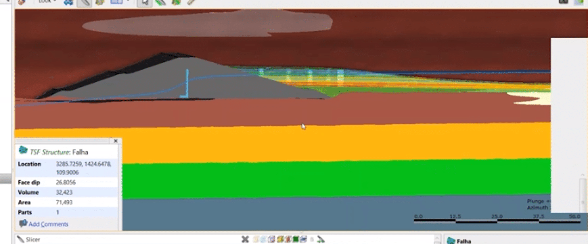
Now, if I click on this fault structure,

[00:16:44.860]
I could turn that off real quick,

[00:16:46.180]
and we can see that there is a very clear

[00:16:48.700]
fault or fracture zone indicated on the geophysical survey,

[00:16:53.040]
which is essential to understanding potential seepage issues

[00:16:58.140]
at this dam site.

[00:17:01.370]
Now from the 2D grids that we have collected

[00:17:08.120]
at this case study,

[00:17:09.880]
we can actually create a 3D model

[00:17:13.470]
of the numeric data within Leapfrog.

[00:17:17.120]
So this 3D model that we were now seeing here

[00:17:19.900]
was collected directly from the numeric data

[00:17:25.190]
that was imported into Leapfrog from Oasis Montage.

[00:17:29.690]
Now there’s a variety of different applications

[00:17:31.750]
for numeric models in Leapfrog,

[00:17:33.080]
whether this is a permeability model,

[00:17:35.910]
in this case, an electrical resistivity model,

[00:17:38.950]
but there’s a lot that you can do with these in Leapfrog,

[00:17:41.980]
such as evaluating these onto cross-sections

[00:17:44.980]
and/or determining actual volumes of material

[00:17:47.910]
that might be over or under a certain interval.

[00:17:54.800]
Now, one of the areas where we can save you the most time

[00:18:00.460]
in your dam monitoring and modeling workflow

[00:18:04.200]
is by creating very quick and rapid dynamic cross-sections

[00:18:08.340]
within Leapfrog.

[00:18:09.990]
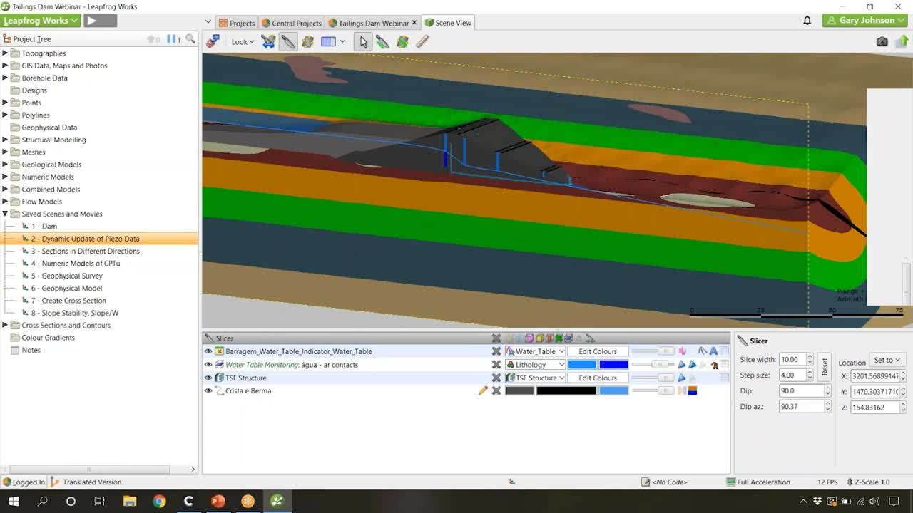
So here I have a saved scene with the geologic model

[00:18:14.850]
and the slicing tool applied,

[00:18:17.100]
and I’m going to show you

[00:18:17.990]
how quick we can make a cross-section within Leapfrog.

[00:18:23.340]
Now, everything in Leapfrog,

[00:18:26.130]
all of the edits are done within the project tree.

[00:18:30.250]
Everything that can be created can be done

[00:18:32.450]
by just right-clicking on a folder in Leapfrog,

[00:18:34.710]
so for example,

[00:18:35.543]
here we’re going to be making a cross-section,

[00:18:37.500]
so I’ll want to right-click

[00:18:38.880]
on the “Cross-sections and Contours” folder,

[00:18:42.280]
and for this example, I’ll be making a new cross-section.

[00:18:47.900]
Now you can see on the section that we have an F and a B,

[00:18:53.020]
and this actually corresponds to the Front and the Back

[00:18:55.750]
of the section.

[00:18:56.910]
So right now I have the F facing me,

[00:18:59.410]
this will be the front of the section, and that is correct.

[00:19:01.570]
Now if you ever had the B facing you

[00:19:03.310]
and you wanted that to be the front,

[00:19:05.040]
you can just choose to swap the front.

[00:19:08.470]
This looks good as is,

[00:19:09.630]
and I’m going to name this “Webinar Section”,

[00:19:15.070]
and I’m going to go ahead and press okay.

[00:19:19.500]
Now if I clear the scene

[00:19:21.330]
and bring the webinar section into the scene,

[00:19:23.420]
we just have the geometry of that section created.

[00:19:27.580]
Now we actually want to go in

[00:19:28.730]
and evaluate our model onto that.

[00:19:31.690]
So I’m going to right-click on Webinar Section

[00:19:34.530]
and choose Evaluations.

[00:19:38.160]
And I’m going to choose the dam structure geologic model

[00:19:42.280]
that we have created,

[00:19:44.670]
and I’m going to go ahead and press okay.

[00:19:53.470]
Now the model has evaluated onto the cross-section

[00:19:58.570]
and using the display tools in the dropdown options,

[00:20:01.410]
we can actually apply the model structure to that.

[00:20:05.530]
So in a matter of seconds,

[00:20:08.300]
we have now created a cross-section

[00:20:10.040]
from the existing geologic model.

[00:20:12.960]
This section can, of course, be exported,

[00:20:17.780]
and if we right-click on the cross-section

[00:20:20.640]
down at the bottom here,

[00:20:21.550]
we can choose to export this

[00:20:24.090]
in a variety of very common export formats,

[00:20:27.250]
such as a DXF, a DWG or a DGM.

[00:20:32.520]
Now if you were going to be running slope stability,

[00:20:35.790]
or seep analysis on the section,

[00:20:39.250]
you can choose to do 2D analysis

[00:20:41.940]
and flatten the section to 2D.

[00:20:46.690]
Now these can then be brought into

[00:20:48.950]
a multitude of different programs,

[00:20:51.020]
specifically, in this case,

[00:20:52.170]
we brought this section into geo studio, in Slope/W,

[00:20:56.370]
to run a slope stability analysis.

[00:21:00.260]
You can also choose to evaluate surfaces onto the section,

[00:21:06.140]
for example,

[00:21:06.973]
you might want to evaluate a water level surface

[00:21:09.580]
onto this section as well.

[00:21:13.430]
Now after that had been exported to Slope/W

[00:21:17.300]
and the geo-technical analysis was conducted,

[00:21:20.520]
that can also then be re-imported

[00:21:22.640]
back into the cross-sections and contours folder

[00:21:25.810]
by right-clicking

[00:21:27.290]
and importing a new cross-section from image.

[00:21:32.040]
Here we have imported that section back in

[00:21:34.740]
after running the analysis, which you can see here,

[00:21:38.270]
and we have combined this in the Leapfrog 3D scene

[00:21:41.230]
with the geologic model.

[00:21:45.510]
And this is essential to show

[00:21:47.200]
that you can then bring everything back into the same space

[00:21:50.880]
to not only analyze your geologic model,

[00:21:53.920]
but also the slope stability analysis

[00:21:55.970]
that you have run in the 3D environment.

[00:22:00.830]
By bringing in the slope stability analysis,

[00:22:04.770]
we have completed the workflow.

[00:22:08.370]
We can now see everything

[00:22:09.870]
in the Leapfrog modeling environment

[00:22:12.950]
from geophysical data and a numeric model

[00:22:16.440]
to a geologic model, cross-sections,

[00:22:20.120]
and then our geo-technical analysis

[00:22:22.190]
that has then been applied to those cross-sections.

[00:22:26.800]
Now, how do you communicate the challenges or the risks

[00:22:31.610]
involved with monitoring and modeling a dam?

[00:22:35.550]
For that, of course, you can export cross-sections

[00:22:38.340]
from Leapfrog in common format, such as a PDF,

[00:22:41.110]
which can be included on a report,

[00:22:43.520]
but we have also created Sequent Central,

[00:22:47.420]
which is our cloud-based model management

[00:22:49.860]
and collaboration solution,

[00:22:51.840]
which allows me to share work in 3D

[00:22:54.780]
with colleagues, clients, and stakeholders,

[00:22:58.510]
as well as it allows you to create conversations

[00:23:03.030]
and to communicate risks involved in 3D.

[00:23:07.260]
So I will now jump into our Central browser.

[00:23:16.240]
The Central browser allows you to see the objects in 3D,

[00:23:21.400]
it allows you to interact with them as well,

[00:23:25.160]
but you don’t actually have the ability

[00:23:27.140]
to go in and edit anything.

[00:23:28.460]
So this is a great way to share your work with stakeholders

[00:23:32.166]
and/or project managers,

[00:23:34.420]
and to keep others involved in the project,

[00:23:36.820]
though they might not actually be involved

[00:23:38.920]
in the 3D modeling process.

[00:23:42.750]
Now on the right here,

[00:23:43.750]
you can see that I’ve created annotations,

[00:23:46.840]
anyone who is also on the Central server,

[00:23:50.310]
who you have added to it

[00:23:51.920]
and given them permission to this project

[00:23:54.150]
can also add or reply directly to comments

[00:23:58.100]
that you have created.

[00:23:59.940]
Now, something cool that I’ve done here

[00:24:01.460]
is that I’ve also created geotags

[00:24:04.430]
so that you can tell a story

[00:24:06.650]
and focus the conversation on a single location.

[00:24:10.480]
So these geotags

[00:24:11.880]
will actually bring you directly to that perspective.

[00:24:14.120]
If I click on one of the comments,

[00:24:20.120]
it’ll take me directly to the location

[00:24:21.970]
where I first saved that comment and made some annotations.

[00:24:26.280]
This is a great way to communicate challenges

[00:24:29.330]
and/or identify potential areas of interest

[00:24:32.210]
within your project,

[00:24:34.360]
while also maintaining a clear auditable history

[00:24:38.150]
of that project.

[00:24:39.970]
Now, this is essential for dam monitoring

[00:24:43.770]
because we all know the risks involved

[00:24:46.070]
in creating a dam of any type,

[00:24:48.680]
whether this is a tailings dam

[00:24:50.360]
for the mining and mineral industry,

[00:24:52.200]
and/or a dam for water resources,

[00:24:54.660]
which is supplying water to individuals, such as myself.

[00:25:00.950]
Dam failure can be catastrophic

[00:25:03.580]
and ensuring dam safety is one of the most important things,

[00:25:08.430]
if not by far the most important

[00:25:11.040]
in a dam projects life cycle,

[00:25:13.070]
everything from design phase to the actual monitoring phase

[00:25:17.540]
after the dam has been constructed.

[00:25:22.551]
<v Mikayla>Thank you Gary,</v>

[00:25:23.384]
and thank you everyone for attending today’s webinar.

[00:25:26.900]
If you have any other questions,

[00:25:28.610]
please contact our technical support team

[00:25:30.640]
at [email protected]

[00:25:34.690]
On behalf of Sequent,

[00:25:36.010]
thank you for joining us and have a great rest of your day.