Oasis montaj & Leapfrog Geo: interoperability workflows (Remote Roundup 2021)

Come see data exchange workflows and how to collaborate and share your Geophysical and Geological modelling efforts.

Overview

Video Transcript

[00:00:00.639]
(soft music)

[00:00:10.629]
<v Geoff>Good morning and good afternoon</v>

[00:00:11.880]
for everyone in attendance.

[00:00:13.600]
Thank you very much for joining.

[00:00:15.700]
Thank you for taking time out of your day

[00:00:17.220]
and joining us for this presentation.

[00:00:19.370]
Today we’re going to be looking at Interoperability Workflows

[00:00:22.130]
between Oasis montaj and Leapfrog Geo

[00:00:25.090]
enabled through Central.

[00:00:28.000]
So just as a quick introduction,

[00:00:29.870]
my name is Geoff Plastow and I’m a Senior Geophysicist

[00:00:33.410]
here at Seequent,

[00:00:34.844]
and I’m based in Vancouver, British Columbia.

[00:00:37.450]
The majority of my professional experience

[00:00:39.500]
is in mining exploration,

[00:00:41.320]
but I’ve worked on several civil

[00:00:43.190]
and an environmental projects

[00:00:45.040]
using geophysics to map voids, groundwater,

[00:00:47.970]
and contributions to earthquake hazard analysis.

[00:00:52.240]
As you can imagine from the title of this presentation,

[00:00:54.980]
we will be demonstrating some key workflows

[00:00:57.210]
and how to effectively collaborate on geoscience projects.

[00:01:01.660]
Today I’ll be working across three

[00:01:03.600]
Seequent software applications,

[00:01:05.890]
Leapfrog Geo, Oasis montaj and Central.

[00:01:10.430]
For those in the audience who are also using Target,

[00:01:13.400]
the same workflow is generally applicable.

[00:01:19.780]
So before we jump into the software,

[00:01:22.150]
I’m just going to provide you a quick introduction to Central.

[00:01:25.250]
Central is a cloud-based data and model management solution

[00:01:29.520]
that allows you and your team

[00:01:31.330]
to work from a single source of truth.

[00:01:34.180]
Through Central project stakeholders,

[00:01:36.640]
whether you’re an active modeler,

[00:01:38.690]
reviewing or third parties,

[00:01:40.610]
such as consultants or JV partners,

[00:01:43.150]
you’ll have access to the latest information

[00:01:45.400]
and intelligence.

[00:01:46.800]
This allows you to inform yourself on the next steps

[00:01:49.730]
for your geoscience project.

[00:01:54.167]
The key to Central is that it provides a means to work

[00:01:57.170]
effectively and efficiently in a multidisciplined team.

[00:02:01.400]
This way we can make a robust and holistic earth model.

[00:02:06.210]
Central enables us to instantly communicate

[00:02:08.560]
the latest results to our team.

[00:02:13.350]
So how does Central actually work?

[00:02:16.210]
Central is a cloud hosted solution hosted by Microsoft

[00:02:19.820]
and administered by us.

[00:02:21.700]
There’s three different access gateways that we can use

[00:02:24.770]
to access information on Central.

[00:02:27.400]
We have our desktop products,

[00:02:29.260]
which you might be familiar with, Leapfrog Geo Works,

[00:02:32.540]
Geothermal, Oasis montaj, Target and Growing.

[00:02:36.710]
This allows us to download

[00:02:38.570]
and publish models and data from Central.

[00:02:41.350]
We can integrate meshes and grids

[00:02:43.240]
and interact with the data room

[00:02:45.450]
and we can receive and reply to comments

[00:02:48.260]
from our colleagues.

[00:02:50.440]
There’s also the Central browser,

[00:02:52.230]
which is a desktop application.

[00:02:54.250]
This is a communication platform.

[00:02:56.830]
It allows us to actively engage with the modeling process,

[00:03:00.260]
we can look at annotations,

[00:03:01.680]
we can review and compare models,

[00:03:03.540]
and we can explore a variety of objects.

[00:03:06.160]
We’re going to be working at the Central browser today.

[00:03:09.189]
And then we have the Central portal,

[00:03:10.910]
which is a web application.

[00:03:12.850]
We can receive and set real time notifications.

[00:03:15.790]
We can download and publish data to the data room

[00:03:18.360]
and we can manage our users

[00:03:19.820]
to see who can access information in our projects.

[00:03:27.000]
The workflow I’d like to demonstrate today

[00:03:28.760]
is more or less summarized by this diagram.

[00:03:31.240]
And it’s how Central can be used

[00:03:32.800]
in an iterative modeling process.

[00:03:35.780]
The data we’re looking at today

[00:03:37.170]
is an early stage geological model

[00:03:39.470]
developed in Leapfrog Geo.

[00:03:41.300]
Here, we can take various types of spatial

[00:03:43.450]
and numerical data,

[00:03:44.960]
things like drilling, mapping, arsenic values.

[00:03:47.670]
And we can develop an initial interpretation of our geology.

[00:03:51.450]
These findings can be published

[00:03:53.410]
and communicated through Central.

[00:03:55.980]
Here, a geophysicist can interact with this data

[00:03:59.430]
and export the required files or hypotheses

[00:04:03.810]
and work with them in Oasis montaj

[00:04:05.960]
and perform geophysical modeling.

[00:04:08.120]
Then in turn publish these results back to Central.

[00:04:12.340]
The idea here is rinse and repeat

[00:04:14.910]
to develop an iterative

[00:04:16.250]
and more communicative modeling process.

[00:04:20.490]
So now, I’m going to jump into the software and do a live demo.

[00:04:32.912]
So we’re going to begin our journey in the Central browser.

[00:04:36.410]
On the left-hand side of the screen,

[00:04:38.320]
you can see all of the Central servers

[00:04:40.470]
that you have available to your organization.

[00:04:43.630]
Now, these are connected to your Seequent ID.

[00:04:45.910]
So when you sign in with your Seequent ID

[00:04:47.640]
to the Central browser,

[00:04:49.380]
you will automatically be authenticated to the servers

[00:04:52.980]
and you’ll see what projects

[00:04:54.472]
you have available to you as well.

[00:04:56.680]
In this case, I’m going to be working

[00:04:57.910]
on this Mt Palmer project.

[00:04:59.900]
I can simply click on it to open the history of the project.

[00:05:05.260]
On the left-hand side of the screen,

[00:05:07.180]
we see a history of the product revisions,

[00:05:09.510]
the project stage, who was published it and some comments.

[00:05:15.730]
On the right-hand side of the screen,

[00:05:17.420]
we can look at the revisions and we can see metadata.

[00:05:21.720]
We can see the various objects inside of the model.

[00:05:25.970]
We can see some of the metadata

[00:05:27.860]
and comments that go along with it.

[00:05:30.500]
We can click on some of the drilling information

[00:05:32.800]
to see the number of colors, the drilling length,

[00:05:36.470]
and some information about arsenic and gold

[00:05:39.150]
that has been logged in those drill holes.

[00:05:42.690]
We can also see an ongoing conversation

[00:05:44.750]
between myself and my colleague, Stephen Donovan.

[00:05:48.860]
So let’s take a look and I’m going to hover over

[00:05:50.930]
and click on one of these thumbnails.

[00:05:52.830]
And it’s going to open up the project in a seen view.

[00:06:00.170]
As I mentioned earlier,

[00:06:01.050]
this is an early stage exploration project.

[00:06:04.190]
We’re looking for a banded iron formation,

[00:06:07.030]
and we’ve also performed a small geophysical survey.

[00:06:10.220]
And what we’re looking at now are the geophysical results.

[00:06:14.720]
We see the areas of a high magnetic intensity

[00:06:17.460]
in pink and red,

[00:06:18.730]
and the areas of a low magnetic intensity in blue.

[00:06:22.450]
So we’ve identified this structure

[00:06:24.900]
and we’ve actually drilled it eight times.

[00:06:29.000]
And my colleague, Stephen has come up with an addition,

[00:06:32.260]
an initial hypothesis about some

[00:06:34.530]
of the subsurface structure.

[00:06:36.750]
The first hypothesis is that we have a fault

[00:06:40.050]
and the banded iron formation is in this fault structure.

[00:06:46.930]
My colleague Stephen has also indicated that

[00:06:49.510]
he’s also modeled another potential hypothesis

[00:06:52.050]
hypothesis, number two,

[00:06:54.180]
that he’s modeled and anticline structure.

[00:06:57.410]
Now, both of these models, geological models

[00:07:01.790]
fit the drilling results.

[00:07:03.770]
The reality is we’ve only drilled eight holes,

[00:07:05.900]
so we don’t have a great understanding of the structure.

[00:07:09.270]
Is it this dipping structure or is it this anticline model?

[00:07:13.530]
And he’s asking me,

[00:07:14.447]
“Hey Geoff, can you incorporate

[00:07:16.960]
some of the geophysics here

[00:07:18.070]
to perhaps guide some of our next steps

[00:07:20.900]
in our drilling program?”

[00:07:22.700]
So I can simply click reply here.

[00:07:25.030]
And if I want, I can use the @ symbol

[00:07:27.620]
and I can text even in a comment.

[00:07:30.550]
I can say, yes, I’ll take a look

[00:07:34.440]
or I can be a little bit more descriptive in my response.

[00:07:37.560]
So Stephen will be notified

[00:07:38.870]
that I’m now taking a look at his project.

[00:07:42.610]
The first thing I’m going to do as a geophysicist

[00:07:45.180]
is I’m going to look at the two,

[00:07:48.750]
the two structural models that we can perform

[00:07:51.230]
geo-physical modeling on.

[00:07:53.100]
I’m going to right click

[00:07:54.610]
and I’m going to simply export this model.

[00:07:58.840]
I’m primarily interested in the banded iron formation

[00:08:01.280]
that he has modeled.

[00:08:03.660]
And I select this model and I select this

[00:08:06.750]
as our anticline model.

[00:08:08.750]
And I say export, and I’m just going to export it.

[00:08:13.650]
And I can repeat this exact same process

[00:08:16.620]
for our dipping fault model.

[00:08:21.850]
So I can simply right click on it

[00:08:25.110]
and export it as a Leapfrog model file.

[00:08:28.070]
There’s a number of other formats that we can export as

[00:08:30.510]
in this case,

[00:08:31.343]
I’m comfortable using Leapfrog model file formats.

[00:08:35.530]
So once I’ve exported these two, these two meshes,

[00:08:39.560]
I’m going to jump into Oasis montaj.

[00:08:44.660]
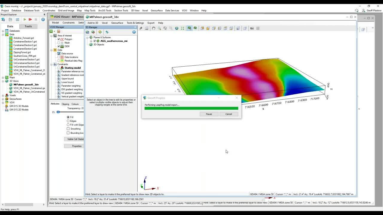
So here we are inside of Oasis montaj,

[00:08:48.080]
I’m visualizing the magnetic data

[00:08:49.970]
that we collected over the survey area,

[00:08:52.440]
and what I’m going to do now

[00:08:53.570]
is I’m going to import the two different

[00:08:55.980]
geological hypotheses.

[00:08:58.430]
First, I’m going to import our dipping plate model,

[00:09:13.120]
and I’m just assigning a geographical projection to that.

[00:09:18.990]
So here’s our dipping plate model,

[00:09:20.520]
and next I’m going to import our anticline model.

[00:09:31.400]
Now, if you haven’t used Oasis montaj before,

[00:09:34.500]
Oasis montaj is a geoscience platform

[00:09:37.960]
that allows you to integrate all types of geoscience data.

[00:09:41.710]
In this case,

[00:09:42.543]
we’re going to be working with geophysical data

[00:09:44.550]
and we’re going to perform some geo-physical modeling

[00:09:47.550]
to test these different hypothesis.

[00:09:50.240]
We’re going to perform a geo-physical forward model

[00:09:53.730]
of the anticline model.

[00:09:55.690]
And then we’re going to perform a forward model

[00:09:58.430]
of this dipping plate model.

[00:10:01.170]
Now, what is the forward modeling process?

[00:10:04.180]
Well, the forward modeling process

[00:10:05.960]
is when we know what is in the ground.

[00:10:08.550]
In this case, we know we have an anticline or dipping model.

[00:10:11.700]
We have these two hypotheses,

[00:10:13.780]
we assign a physical rock property to it,

[00:10:16.190]
and then we calculate what the magnetic response looks like.

[00:10:20.900]
So what we’re going to do is we’re going to calculate

[00:10:22.980]
the forward response from both of these,

[00:10:25.340]
and then compare it with our data.

[00:10:27.330]
And we’re going to just make a qualitative assessment

[00:10:29.580]
as to which one of these

[00:10:31.180]
most matches the chief physical data.

[00:10:34.840]
So I’ve already gone ahead and I’ve created a geo-physical

[00:10:38.430]
modeling space inside of VOXI,

[00:10:40.650]
and the extensive of this is our project area.

[00:10:44.900]
The next thing I’m going to do is I’m going to add

[00:10:47.420]
a starting model constraint.

[00:10:49.620]
So I click create and build a model.

[00:10:53.800]
I can, I’m going to start off with the dipping plate model.

[00:10:57.180]
I’m going to select a starting model.

[00:10:59.830]
The surface I’m going to use,

[00:11:01.370]
I’m going to use the dipping plate first.

[00:11:04.320]
When I do this again,

[00:11:05.220]
I’m going to use the anticline surface.

[00:11:08.290]
So outside of the area,

[00:11:10.090]
I’m going to assign zero magnetic susceptibility.

[00:11:13.810]
Inside of the dipping plate.

[00:11:15.890]
I’m going to assign a magnetic susceptibility of one.

[00:11:19.600]
We know this from drilling.

[00:11:20.900]
We have some ideas of what some of the physical

[00:11:23.070]
rock properties are.

[00:11:25.130]
When I’m ready, I can click okay.

[00:11:27.520]
And it will create a voxel or geo-physical block model

[00:11:32.740]
that represents this dipping prism.

[00:11:37.360]
If I want, I can use the clipping tool in Oasis montaj

[00:11:40.590]
to see that it is in fact, the dipping plate.

[00:11:45.540]
And once I’m ready,

[00:11:46.373]
I can go ahead and run the forward model.

[00:11:49.910]
To do that, I can just say, run forward model.

[00:11:53.190]
The nice thing about VOXI is that it uses cloud computing.

[00:11:57.210]
It uses Microsoft Azure to do these calculations.

[00:12:01.410]
So the geophysical modeling process

[00:12:03.240]
is quite computationally intensive.

[00:12:06.460]
So by using the Cloud, we get the result much faster.

[00:12:11.040]
And also it doesn’t use any of my computer resources.

[00:12:16.140]
Now for the sake of this webinar,

[00:12:18.020]
I’ve already done the forward calculation

[00:12:20.080]
for both the dipping prism and the anticline model.

[00:12:24.300]
So let’s take a look at both of these.

[00:12:27.440]
This here is the forward calculated response

[00:12:30.420]
of the anticline model.

[00:12:34.720]
And on the right-hand side of the screen,

[00:12:36.880]
I have the forward calculating response

[00:12:39.190]
from the dipping prism.

[00:12:42.240]
Now, if we compare this to our magnetic data

[00:12:46.020]
that we acquired over the project area,

[00:12:48.630]
we can simply make a qualitative assessment.

[00:12:51.350]
Does our magnetic data look like the anticline model?

[00:12:54.630]
Well, perhaps we have this broad structure and yes,

[00:12:57.550]
it tapers a little bit to the south,

[00:13:00.080]
but let’s compare our acquired magnetic data

[00:13:03.100]
to the forward calculated response from the dipping prism.

[00:13:06.560]
Again, we see this broad magnetic response tapering.

[00:13:11.550]
Yes, we see some of the highs where we have our highs.

[00:13:14.360]
So from a qualitative point of view,

[00:13:16.860]
we can make an initial assessment and say,

[00:13:19.310]
geophysically physically speaking

[00:13:20.330]
this dipping prism seems to be more geophysically

[00:13:23.390]
plausible at this stage.

[00:13:25.500]
So that’s great.

[00:13:26.730]
We’ve already done a forward calculation

[00:13:28.450]
and we’re leaning towards one of the hypotheses

[00:13:31.240]
and we can perhaps make some decisions

[00:13:33.650]
about how we want to do our next stages of drilling.

[00:13:39.400]
So to continue on this process,

[00:13:41.710]
we can now perform a geophysical inversion.

[00:13:45.190]
So the inversion is the inverse process

[00:13:48.190]
of the forward calculation.

[00:13:50.360]
This means we’re going to take our geophysical data

[00:13:53.630]
and we are going to produce a block model or a voxel

[00:13:58.110]
of physical rock properties.

[00:14:02.180]
So we are going to move forward with this dipping prism.

[00:14:05.350]
And instead of running a forward model,

[00:14:08.090]
I’m going to run an inversion.

[00:14:10.450]
And again, this data is uploaded to the cloud.

[00:14:13.830]
The calculations will happen in the cloud,

[00:14:15.770]
so my computer is free and it’s not being bogged down

[00:14:19.000]
by numerical computations and calculations.

[00:14:22.690]
Now, again, for the sake of this webinar,

[00:14:24.470]
I’ve gone ahead and performed the inversion

[00:14:29.380]
and I’ve produced several sections

[00:14:33.480]
through this geophysical inversion.

[00:14:36.430]
And we also have a voxel which represents the distribution

[00:14:41.070]
of magnetic susceptibility in the subsurface.

[00:14:45.250]
This is great.

[00:14:46.330]
Now, how can I share these results with my colleague?

[00:14:48.830]
How can I share these back with Stephen?

[00:14:51.460]
Well, there’s a few ways we can do this,

[00:14:54.670]
in the data services menu

[00:14:56.380]
we can simply upload these results to Central.

[00:15:02.040]
The first thing I’m doing is I’m just ensuring I’m connected

[00:15:05.040]
to the correct Central server.

[00:15:08.600]
I’m going to select the project

[00:15:10.230]
that I want to upload my data to.

[00:15:13.470]
We have the option of uploading our data as OMF,

[00:15:17.960]
OMF is an acronym that stands for Open Mining Format.

[00:15:22.950]
This is an open file exchange format

[00:15:25.390]
that is not directly linked to Seequent software.

[00:15:28.650]
It is an open format that can be digested by many software

[00:15:31.550]
applications and allows you to transfer your data freely.

[00:15:36.650]
So I’m going to select my constraints, susceptibility voxel,

[00:15:40.000]
and I’m going to upload it as an OMF format.

[00:15:43.930]
I can click okay.

[00:15:45.780]
And the export and upload process will start.

[00:15:52.510]
This may take a second,

[00:15:53.550]
depending on my internet connection speed.

[00:15:59.360]
So now it’s uploading this result to the Central server

[00:16:02.940]
and it has been uploaded.

[00:16:06.270]
Now I’ve also created some section grids.

[00:16:09.210]
If I want, I can simply go back to the data services menu,

[00:16:12.890]
or I can select these grids from the Project Explorer.

[00:16:16.500]
I can say, right click on the grid I want

[00:16:18.610]
and say upload to Central.

[00:16:22.610]
So here I can upload my individual grids,

[00:16:25.110]
I can select multiple grids if I want.

[00:16:26.920]
Here I’ve created three section grids,

[00:16:28.840]
and I’m going to say, okay,

[00:16:30.250]
and again, these are going to upload to our Central project.

[00:16:39.040]
So what I’m going to do now,

[00:16:40.270]
while this is just finishing uploading,

[00:16:42.050]
I’m going to jump into Leapfrog Geo.

[00:16:48.010]
So here we are at Leapfrog Geo.

[00:16:49.940]
We have our magnetic survey results,

[00:16:53.860]
and we can go ahead and now begin to import these results,

[00:16:57.570]
these geophysical inversion results into Leapfrog Geo.

[00:17:01.370]
So I could go to the geophysical data folder, right click,

[00:17:04.880]
and we have two options.

[00:17:06.150]
We can import the grid as a standalone file

[00:17:08.410]
in case it just lives on your hard drive.

[00:17:10.530]
In this case, I’m going to import these 2D grids from Central.

[00:17:15.560]
I’m going to select my Central project.

[00:17:19.120]
I can see all of the branches and the geophysical data

[00:17:22.990]
that’s already been downloaded.

[00:17:25.320]
If I jump into files into the data room,

[00:17:27.810]
I can see that these are the files that we’ve updated.

[00:17:31.290]
So I can select these grids and say, import.

[00:17:36.270]
This process may just take a second,

[00:17:37.740]
depending on your internet connection speed.

[00:17:41.720]
But once the download is finished, the grid is available

[00:17:45.550]
and can be dragged into your model space.

[00:17:50.940]
What’s really great is that the greatest, correctly oriented

[00:17:56.060]
it’s correctly geo-referenced,

[00:17:58.160]
and the color distribution that I used in Oasis montaj

[00:18:01.580]
is transferred to Central

[00:18:03.170]
and then down into Leapfrog Geo.

[00:18:06.380]
So we don’t have to worry about any discrepancies

[00:18:08.420]
about the way things look and feel.

[00:18:10.990]
Now, what about the geophysical block model,

[00:18:13.010]
the voxel we created.

[00:18:14.690]
Again, if I want I can import the OMF as a direct file

[00:18:18.900]
from my hard drive,

[00:18:20.010]
or I can import it from Central.

[00:18:21.970]
Again, I’m going to pick the project I want,

[00:18:24.930]
I’m going to select the OMF file of interest,

[00:18:30.040]
going to import this.

[00:18:34.760]
Again, this is just processing

[00:18:36.950]
and again, I can just drag it into my model space.

[00:18:41.200]
Now, one of the first things that we see is yes,

[00:18:43.620]
perhaps the color distribution of the OMF file

[00:18:46.230]
did not carry over.

[00:18:47.740]
Well, a quick work around for that is we can take our grid,

[00:18:52.270]
our grid object,

[00:18:53.860]
and we can just export the color map for this.

[00:18:58.760]
So I’m going to call this the magnetic susceptibility

[00:19:01.380]
color map.

[00:19:03.110]
And once that has been created,

[00:19:05.510]
we can go ahead and import this, import this color map

[00:19:12.590]
from the gridded section,

[00:19:17.050]
and then we can now apply it to our voxel data.

[00:19:21.645]
And what’s great is now we have our geophysical data,

[00:19:24.220]
our sections, and our geophysical volumes,

[00:19:27.000]
physical rock properties inside of Leapfrog Geo.

[00:19:29.710]
And we can continue to iterate on this modeling cycle.

[00:19:33.400]
We can now continue to integrate this

[00:19:35.073]
into our geological model

[00:19:36.670]
and perhaps make decisions about how we do our drilling.

[00:19:44.530]
So just jumping back into PowerPoint,

[00:19:47.410]
I just wanted to reiterate that we can use Central,

[00:19:52.640]
Leapfrog Geo and Oasis montaj and Target

[00:19:55.720]
in an iterative, collaborative, modeling process.

[00:19:58.860]
We can use it as a communication tool to effectively share,

[00:20:02.210]
track and collaborate our changes

[00:20:03.870]
through the modeling process.

[00:20:06.010]
So you can see how the next set of drilling results again,

[00:20:09.610]
we can insert these into the feedback,

[00:20:12.370]
recalculated geo-physical model,

[00:20:15.050]
and then provide that back to the geoscience team.

[00:20:20.780]
So this concludes my demonstration and presentation

[00:20:23.930]
this morning.

[00:20:25.480]
If we have…

[00:20:26.313]
We have a few minutes for any questions that you might have.

[00:20:34.050]
<v Stephen>Yeah, hi.</v>

[00:20:35.280]
My name’s Stephen Donovan as well,

[00:20:36.460]
so I’m going to be helping Jeff with the questions.

[00:20:38.890]
If you have anything, please enter that into the chat now,

[00:20:42.190]
and we’ll be happy to feel both.

[00:20:47.690]
We did have one question here around supported file types.

[00:20:52.090]
Can you speak to what kind of data you can transfer

[00:20:55.310]
between Oasis and Leapfrog, Geoff?

[00:20:58.600]
<v Geoff>Yeah, that’s a really good question, Stephen.</v>

[00:21:01.940]
So I mentioned Oasis montaj and Target itself.

[00:21:04.890]
I can work with them for such a wide variety of data sets.

[00:21:08.170]
In this example, I used geophysical data

[00:21:11.370]
and I did some geophysical modeling,

[00:21:13.180]
but this whole process could be done with geochemical data

[00:21:16.550]
or even surficial soil sampling, XRF data, solidity levels,

[00:21:21.940]
resistivity data.

[00:21:22.773]
So there’s really no limitation on numerical data

[00:21:27.670]
that can be shared through Central

[00:21:31.060]
and then integrated into a Leapfrog project.

[00:21:36.950]
<v Stephen>Great, and then what about licensing costs?</v>

[00:21:40.360]
Are there any license costs

[00:21:42.570]
associated with connecting Oasis montaj to Central?

[00:21:48.620]
<v Geoff>That’s a good question.</v>

[00:21:49.640]
So at this time,

[00:21:50.970]
if your organization has a Central server,

[00:21:53.910]
there is no associated cost with connecting Oasis montaj

[00:21:57.330]
or Target to that server.

[00:22:00.350]
And that will allow you to access that information

[00:22:03.110]
in the exact same way that you saw today.

[00:22:05.270]
I can publish models,

[00:22:06.410]
I can use the Central browser to view and export

[00:22:09.500]
models and meshes,

[00:22:10.470]
and then pull those into Target in Oasis montaj

[00:22:13.180]
and be part of the iterative model,

[00:22:14.013]
my iterative modeling cycle.

[00:22:18.100]
<v Stephen>That’s fantastic.</v>

[00:22:20.570]
So we don’t see any other questions coming up.

[00:22:22.980]
If you do have any feel free to type them in there,

[00:22:29.140]
otherwise back over to you, Geoff to wrap up.

[00:22:31.730]
<v Geoff>Yeah, sure.</v>

[00:22:33.260]
I just want to thank everyone for their time today.

[00:22:35.280]
We appreciate you taking the time out of the day

[00:22:36.800]
to watch the presentation.

[00:22:38.310]
If you have any questions about what you saw today,

[00:22:40.400]
feel free to reach out to myself,

[00:22:42.620]
my email address is here on the screen.

[00:22:45.042]
And if you’re interested in a trial or demo

[00:22:46.800]
of Leapfrog Geo, Oasis montaj or Central,

[00:22:50.010]
we can certainly assist with that as well.

[00:22:51.840]
So thank you very much for your time.

[00:22:55.130]
Bye for now.

[00:22:58.562]
(soft music)