Oasis montaj 9.10 – Release Highlights

We have listened to your feedback, improved performance and optimized workflows whilst streamlining extensions and adding more flexibility and interoperability.

Experience a much more comprehensive, intuitive, and easier to use Projections & Coordinate System, supporting more standard projects and powerful new search functionality.

We’ve renamed and revamped the IP and Resistivity Extension to Induced Polarization & Resistivity – expect better visualization, better QC and better processing workflows.

Focused on increasing your functionality and usability, the UX-Analyze extension also has a new intuitive menus.

Video Transcript

[00:00:00.198]
(calming music)

[00:00:10.220]
<v Laura>Hello, my name is Laura Quigley</v>

[00:00:12.360]
and I’m a technical analyst here at Seequent.

[00:00:15.600]
I’m going to share with you some of the new features

[00:00:17.820]
in the June, 2021 release of Oasis montaj version 9.10.

[00:00:24.670]
This release is a scheduled software upgrade

[00:00:26.680]
available to all maintain customers

[00:00:28.470]
and can be downloaded from myseequent.com.

[00:00:32.530]
First, I will cover a few items

[00:00:34.450]
so that you know how to participate in today’s webinar.

[00:00:38.500]
During the webinar, you will have the option

[00:00:40.110]
to submit text questions by typing your questions

[00:00:42.157]
in the chat pane of the GoToWebinar panel.

[00:00:45.950]
You may send your questions at any time

[00:00:47.470]
during the presentation

[00:00:48.840]
and we will respond to those questions via email

[00:00:50.909]
within the next 24 to 48 hours.

[00:00:56.240]
A faster, more powerful version of Oasis montaj

[00:00:58.830]
is now available in our latest release.

[00:01:01.500]
We have listened to your feedback,

[00:01:03.220]
improved performance and optimized workflows

[00:01:06.270]
while streamlining extensions

[00:01:08.300]
and adding more flexibility and interoperability.

[00:01:12.390]
An overview of some of the features

[00:01:13.670]
that we’ll be discussing include,

[00:01:15.660]
how the user will experience a much more comprehensive,

[00:01:18.170]
intuitive, and easier to use projection

[00:01:20.060]
and coordinate systems.

[00:01:22.430]
We’ve also renamed and revamped the IP extension

[00:01:25.440]
to IP and Resistivity.

[00:01:27.470]
We’ve made some customer usability requests,

[00:01:30.540]
such as better handling of lost data files

[00:01:33.630]
and the ability to import KML or KMZ vector layers

[00:01:36.840]
into 3D views.

[00:01:39.710]
You can now upload folders to the Seequent Data Room.

[00:01:43.430]
We’ve made frequency domain filtering

[00:01:45.430]
usability improvements.

[00:01:47.110]
We have added two new convolution filters

[00:01:50.580]
and have made updates to our Airborne QC extension.

[00:01:53.690]
There’s also a new intuitive menu structure

[00:01:55.568]
for UX-Analyze workflow.

[00:01:58.010]
And in VOXI, we have a new waveform option

[00:02:00.090]
for time domain EM modeling

[00:02:02.970]
and a new regularization method

[00:02:04.248]
for DCIP, time domain EM

[00:02:06.500]
and frequency domain EM models in VOXI.

[00:02:09.690]
And finally, we have a new DAP URL.

[00:02:12.720]
Coordinate systems and projections.

[00:02:15.990]
We’ve made significant improvements and updates

[00:02:17.880]
to coordinate systems and projections.

[00:02:21.240]
The menu has all the parameters

[00:02:22.600]
of the previous coordinate system dialogue,

[00:02:24.610]
plus a few additions.

[00:02:27.590]
So locating your coordinate system for your project

[00:02:29.248]
has now been made faster and more intuitive

[00:02:31.680]
through our new powerful multi-string search functionality.

[00:02:35.300]
You can now search your coordinate system by country name,

[00:02:38.560]
latitude or longitude

[00:02:40.620]
or standard coordinate system name.

[00:02:43.940]
You can also search by unique EPSG or IOPG code

[00:02:48.330]
or an Esri ID.

[00:02:50.660]
And by using these unique IDs,

[00:02:52.060]
there is no confusion about which version

[00:02:53.850]
of the datum you are using.

[00:02:56.870]
So we show the coordinate system

[00:02:58.290]
in a tree that is multilevel.

[00:03:00.810]
The first level will either be geographic coordinates system

[00:03:03.340]
or projected system.

[00:03:05.610]
The second level is the country,

[00:03:07.430]
as you often know what country you are working in.

[00:03:11.060]
The third level, if broken down further,

[00:03:12.850]
will be your latitude or longitude.

[00:03:16.090]
And the fourth level will show the coordinate system itself.

[00:03:20.100]
You can also search by unique EPSG number, as I mentioned,

[00:03:23.330]
so for example, 4326 is WGS 84 geographic coordinate system.

[00:03:31.860]
We’ve also included several new coordinate projections

[00:03:34.960]
applicable to Antarctica, Scandinavia,

[00:03:37.323]
Papa New Guinea,

[00:03:39.160]
Borneo, Brazil and more.

[00:03:47.170]
So I’m going to click next to create some new channels.

[00:03:51.660]
I’m in Finland zone three,

[00:03:52.980]
so I can begin to type this into the multi-string search.

[00:03:56.850]
I don’t see anything that matches what I’ve typed in

[00:03:59.143]
in my standard list,

[00:04:01.150]
but I do see a note saying

[00:04:02.404]
the Esri coordinate system list does contain a search

[00:04:05.980]
that matched what I typed in.

[00:04:08.010]
We can also add coordinate systems to a favorites tab,

[00:04:11.580]
making it easy to access the coordinate systems

[00:04:14.460]
you use often.

[00:04:15.630]
This is also extremely useful

[00:04:17.010]
if you have custom coordinate systems.

[00:04:20.750]
You can now push the current projected coordinate systems

[00:04:23.040]
to multiple files within your projects,

[00:04:24.700]
such as grids or databases,

[00:04:27.300]
complimentary to the copy from option.

[00:04:31.160]
Further, we have updated the modify dialogue.

[00:04:34.000]
You can now customize a local datum transform.

[00:04:42.170]
All these changes and updates were implemented

[00:04:44.290]
to help you navigate the coordinate system menu

[00:04:46.330]
in Oasis montaj,

[00:04:47.860]
allowing you to save time looking for your desired

[00:04:49.699]
and favorite coordinate systems.

[00:04:55.670]
IP and resistivity.

[00:05:00.310]
Next, I’m going to talk about our IP and Resistivity extension.

[00:05:04.860]
We have renamed this extension from IP

[00:05:07.240]
to IP and Resistivity

[00:05:09.490]
to better describe the functionality

[00:05:11.590]
and the naming is more in line with our VOXI terminology.

[00:05:16.580]
We’ve also improved 2D plan map visualization.

[00:05:20.750]
You can now access contributing electrodes quickly

[00:05:23.640]
via an icon on the title bar.

[00:05:27.620]
You can clearly visualize the contributing electrodes

[00:05:30.480]
for each IP measurement.

[00:05:34.320]
When you are done, use the adjacent button

[00:05:36.090]
on the database toolbar

[00:05:37.570]
to end plotting contributing electrode mode.

[00:05:42.360]
We’ve also updated 3D array plotting.

[00:05:46.830]
We have done two things.

[00:05:49.460]
First, you can now plot symbols scaled by amplitude

[00:05:53.490]
using the proportional radio button.

[00:05:56.610]
And this will minimize the size of low values,

[00:05:59.200]
minimizing clutter in your 3D view.

[00:06:03.820]
Secondly, you can now group layers by line numbers

[00:06:07.130]
or electrode types.

[00:06:08.710]
That’s all transmitters together and all receivers together.

[00:06:13.200]
This helps expanding and contracting the groups

[00:06:15.061]
in the 3D view,

[00:06:17.090]
so you can expand just the types of data you want to look at.

[00:06:23.570]
The data is grouped here by type

[00:06:25.880]
and I’m able to expand just the group I want to look at.

[00:06:31.340]
Also in this update,

[00:06:32.520]
you can edit multiple groups at the same time.

[00:06:36.130]
You can simply select the group of data

[00:06:38.170]
you would like to edit

[00:06:40.270]
and then change the color or the symbol size.

[00:06:43.190]
For example, if I want to change all the transmitter twos

[00:06:45.920]
to a different color and or size.

[00:06:54.810]
We’ve also added new quality control processing tools.

[00:06:59.130]
Identify noisy arrays.

[00:07:01.830]
We can now identify and filter noisy IP channels.

[00:07:06.300]
As you can see, some channels here are noisy

[00:07:08.680]
and should be flagged.

[00:07:13.260]
This tool will fit a polynomial to the IP decay.

[00:07:16.770]
We can specify the order of the polynomial,

[00:07:19.790]
usually an order of three will cover the decay here well.

[00:07:24.380]
Other parameters, including percent fit error,

[00:07:27.430]
so what is the acceptable range

[00:07:29.330]
and values outside that will be flagged?

[00:07:32.700]
Another perimeter mask QC IP threshold.

[00:07:37.300]
So we initially mask the flagged channel IP mask.

[00:07:41.290]
If this number of elements set in this parameter here

[00:07:44.150]
are flagged in the IP mask,

[00:07:46.390]
then we turn off the QCIP channel altogether

[00:07:51.300]
and then finally, we can save the fitted array

[00:07:53.820]
and the error to two new channels.

[00:07:59.920]
So once run, an array viewer window pops up

[00:08:02.280]
where I can see the original and fitted arrays.

[00:08:05.990]
You can move through the data,

[00:08:08.220]
moving through the fiducial or sample number,

[00:08:11.010]
and you can move down the array

[00:08:12.500]
with the values being displayed along the bottom.

[00:08:21.080]
Another QC tool we have updated,

[00:08:23.210]
is the flag or mask data by range.

[00:08:27.860]
So that’s under QC by data range.

[00:08:33.170]
Initially in this tool, we allowed the user

[00:08:35.080]
to specify only one channel to flag.

[00:08:38.090]
However, there have been requests to mask

[00:08:39.850]
by more than one channel.

[00:08:42.010]
Maybe you have a flag channel you want to use

[00:08:43.810]
in conjunction with the VP channel, for example.

[00:08:47.560]
You can also pick and or a or condition.

[00:08:51.940]
The data statistics are shown along the bottom.

[00:08:55.930]
What is the mean and the range of the data?

[00:08:59.810]
You can flag inside or outside a data range

[00:09:03.110]
or flag by absolute value.

[00:09:10.860]
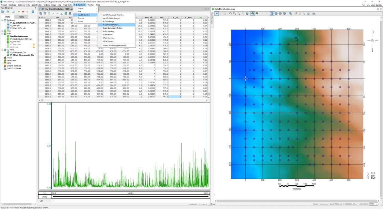
Another tool we have added,

[00:09:12.550]
is QC by data distribution.

[00:09:16.550]
So I’ll open another database to demonstrate this.

[00:09:21.800]
This tool will show you all the receiver values

[00:09:24.260]
related to the same transmitter.

[00:09:29.250]
The top list gives a list of transmitter coordinates.

[00:09:33.120]
Then I can pick a transmitter from the list

[00:09:35.010]
and it will link to the map,

[00:09:37.480]
or I can go to my map and pick a transmitter here.

[00:09:42.000]
Once I pick a transmitter, it shows me all the data values

[00:09:44.930]
and the receiver pairs in the table here.

[00:09:52.320]
What we will normally expect

[00:09:53.530]
is to see higher values closer to the transmitter

[00:09:56.480]
and then drop off as you move further away.

[00:10:01.170]
We can look at these values in the table

[00:10:02.670]
and decide which ones to keep and turn off.

[00:10:07.390]
In the more or less section, we can change the color table

[00:10:11.270]
and the size of the symbols.

[00:10:17.380]
Another new processing tool we have added,

[00:10:19.180]
is recalculate derived data.

[00:10:22.450]
So this was previously called recalculate

[00:10:25.460]
and it would update a group of channels

[00:10:26.853]
that were hardwired or set into the tool.

[00:10:30.560]
Now, you can provide the names of the channels

[00:10:32.383]
instead of using the ones that were hardwired.

[00:10:36.300]
We also allow the user to leave certain fields blank

[00:10:39.430]
that will not be recalculated.

[00:10:44.230]
And finally, we have now added the option

[00:10:46.330]
to calculate the chargeability.

[00:10:51.870]
Customer usability requests.

[00:10:55.160]
Work faster with usability enhancements

[00:10:57.450]
in Oasis montaj and Target.

[00:11:00.640]
In this newest release, you can now manage data in 3D views

[00:11:05.420]
via folders.

[00:11:07.920]
You have the ability to create, rename

[00:11:10.080]
and delete folders and sub folders.

[00:11:13.560]
This allows you to turn data off and on quickly.

[00:11:16.890]
You simply need to drag and drop your content into a folder,

[00:11:19.940]
allowing you to stay organized.

[00:11:23.190]
Seequent Central.

[00:11:25.040]
With this release, we have added the ability

[00:11:26.960]
to upload to folders within the Seequent Data Room.

[00:11:31.340]
You can now create and select folders

[00:11:33.320]
within the Seequent Data Room in which to upload your files,

[00:11:38.060]
making organizing and sharing much smoother.

[00:11:44.490]
In the project explorer,

[00:11:45.770]
we have better handling of lost files and broken data links.

[00:11:50.290]
Now, whenever a file is missing,

[00:11:52.240]
it will be grayed out and a warning sign next to it,

[00:11:55.710]
meaning Oasis montaj cannot locate those files.

[00:11:59.800]
You then have the ability to right button click on the file

[00:12:02.900]
and locate it by choosing find.

[00:12:09.100]
You will also notice the channel grid

[00:12:11.100]
and voxel math tools are significantly faster.

[00:12:14.920]
Finally, we have added the ability to import KMZ

[00:12:18.737]
and KML vector layers into the 3D viewer.

[00:12:32.410]
Frequency domain filtering updates.

[00:12:38.050]
We have made some improvements to our geophysics

[00:12:40.540]
and 2D FFT extensions.

[00:12:43.240]
We had some customer feedback on the 1D

[00:12:45.269]
and 2D FFT filtering in our 9.9 release

[00:12:48.870]
and we acted on that feedback.

[00:12:52.460]
So firstly, in 2D filtering,

[00:12:54.370]
you can now display the filled grid

[00:12:56.860]
without opening the interactive filter definition.

[00:13:00.470]
Here we have added a display button

[00:13:02.270]
that allows you to display the filled grid

[00:13:04.240]
before continuing with the filtering.

[00:13:08.840]
This creates an _PRP grid

[00:13:13.368]
and you can adjust the various parameters,

[00:13:15.300]
such as trend, expansion and fill methods and display

[00:13:18.520]
before running your filter.

[00:13:23.380]
Next, in match filtering,

[00:13:25.160]
we now distinguish between the data

[00:13:27.420]
either being magnetic or gravity data.

[00:13:31.610]
Magnetic values change is one over R queued,

[00:13:35.000]
whereas gravity changes is one over R squared.

[00:13:37.960]
So the way the slope is used

[00:13:39.210]
to calculate the equivalent depth is different.

[00:13:42.520]
So you simply choose the type of data you are working with

[00:13:44.780]
and all the math happens behind the scenes.

[00:13:49.260]
We’ve also made the size of the window

[00:13:51.220]
used to calculate the slope, much bigger,

[00:13:53.870]
so that it’s smoother.

[00:13:55.860]
This is because the spectrum is so noisy.

[00:13:58.030]
Now we can use up to half the length of the spectrum itself.

[00:14:03.920]
And you can see when I go to define the slope

[00:14:05.830]
on the spectrum graph, it moves much smoother.

[00:14:10.100]
We can also change the width of the spectrum for each depth.

[00:14:21.330]
Finally, in the 1D FFT tool, we made a small change

[00:14:24.219]
as to how we display the output spectrum.

[00:14:28.860]
We used to plot the input and output spectrum

[00:14:30.720]
on the same scale,

[00:14:32.430]
however, they can be very different values,

[00:14:34.130]
for example, derivatives.

[00:14:36.490]
So now we plot them separately, such that each profile

[00:14:39.690]
is centered individually on their own midpoint values.

[00:14:46.680]
New convolution filters.

[00:14:49.480]
Next, I’m going to talk about two new convolution filters

[00:14:52.160]
that we have added to version 9.10,

[00:14:54.740]
the vertical continuation convolution filter

[00:14:57.680]
and the Laplacian of Gaussian

[00:14:58.720]
nine by nine convolution filter.

[00:15:02.040]
Both of these filters can be found under grid

[00:15:04.200]
and image filters menu.

[00:15:09.720]
The continuation filter can be used to smooth

[00:15:12.040]
or sharpen your data,

[00:15:13.200]
while the Laplacian can be used to enhance edges.

[00:15:17.130]
The first filter I will speak about

[00:15:18.259]
is the Laplacian of Gaussian,

[00:15:20.070]
a nine by nine convolution filter,

[00:15:22.540]
which yields the second vertical derivative of the data.

[00:15:25.700]
So I’ve run this filter.

[00:15:27.410]
So I will just close this dialog

[00:15:29.010]
and show you the results on my map.

[00:15:35.270]
So here’s the non-filtered magnetic grid

[00:15:38.280]
and the Laplacian grid.

[00:15:53.800]
The second new convolution filter

[00:15:56.310]
is the vertical continuation convolution filter.

[00:16:00.640]
With this filter, we can apply upward

[00:16:02.590]
or downward continuation, with the limitation being

[00:16:05.496]
that you cannot apply the continuation

[00:16:07.630]
by more than five grid cells

[00:16:10.090]
and you will get an error if you try to do so.

[00:16:14.070]
Although this is a limitation,

[00:16:15.171]
you will see that the results can be much cleaner

[00:16:17.760]
than similar FFT method, which is prone to artifacts.

[00:16:22.520]
So first I have the non-filtered magnetic data

[00:16:26.440]
and a grid that was upward continued by 500 meters,

[00:16:31.390]
and this can be run to reduce

[00:16:32.740]
high-frequency short wavelength noise, for example.

[00:16:37.070]
We can also sharpen subtle features

[00:16:38.440]
by applying a downward continuation.

[00:16:41.730]
So here is the vertical continuation convolution filter grid

[00:16:45.320]
that was downward continued 250 meters.

[00:16:50.420]
And just to compare,

[00:16:51.270]
I’ve run a similar downward continuation in the FFT filter

[00:16:57.070]
and I’ll just zoom in to show you the difference.

[00:17:09.160]
Airborne QC.

[00:17:13.070]
Work faster and improve the quality

[00:17:14.750]
of your Airborne geophysics data

[00:17:16.330]
by performing a velocity QC test,

[00:17:19.150]
either individually or by batch.

[00:17:22.000]
This tool flags segments of the survey track

[00:17:24.240]
where velocities are outside the project specifications.

[00:17:28.820]
In the tool, you’ll specify a nominal velocity

[00:17:31.840]
and the allowable range.

[00:17:35.260]
So this produces a flag channel,

[00:17:36.860]
which is then plotted on your map.

[00:17:47.530]
Also, we have made another change to plot QC results,

[00:17:52.470]
where you can customize the appearance of a flag channel.

[00:17:57.190]
If you plot a lot of these QC flags,

[00:17:59.260]
you may find that they are too close to one another

[00:18:01.940]
or over printing one another, for example,

[00:18:04.520]
and you may want to customize the plotting of the QC flags.

[00:18:08.960]
We can now define the offset, color and line thickness

[00:18:12.010]
of the QC flag you want to edit.

[00:18:18.340]
UX-Analyze new menu structure.

[00:18:21.210]
So next, I’m going to jump into PowerPoint

[00:18:23.320]
to talk about the new UX-Analyze menu structure.

[00:18:28.870]
In Oasis montaj version 9.10,

[00:18:30.870]
we have reorganized some of the menus

[00:18:33.410]
in the UX-Analyze workflow.

[00:18:36.510]
We previously had three menus, dynamic data,

[00:18:39.140]
static data and expert user.

[00:18:42.670]
We’ve now broken the tools out into four menus,

[00:18:46.100]
AGC survey prep, dynamic data,

[00:18:48.890]
static data and expert user,

[00:18:51.930]
with AGC in front of the names,

[00:18:53.630]
standing for advanced geophysical classification.

[00:18:58.470]
So the new menu survey prep.

[00:19:02.040]
So this include some of the tools

[00:19:03.135]
that were previously in the dynamic and static workflows.

[00:19:07.700]
So like I said, we’ve moved

[00:19:08.940]
some of these survey preparation tools

[00:19:11.088]
that were previously in the static and dynamic menus

[00:19:15.010]
into a survey prep menu, allowing new users

[00:19:17.559]
or those who do not do AGC processing regularly

[00:19:20.900]
to easily see in these new menus

[00:19:23.720]
what tools are necessary to run respective workflows

[00:19:27.080]
without unnecessary clutter.

[00:19:31.020]
So you’ll see here, I have the old menu on the left

[00:19:33.500]
and the new menu on the right

[00:19:35.760]
for both dynamic and static

[00:19:38.930]
with the new menus being highlighted in a yellow rectangle.

[00:19:44.500]
So the way we restructured this,

[00:19:45.990]
is to include tools that are essential

[00:19:47.870]
to complete the workflow on the main menus.

[00:19:51.380]
So for static data, that would be import static sensor data,

[00:19:55.000]
level sensor data,

[00:19:56.400]
and classify and rank.

[00:19:58.650]
For the dynamic workflow,

[00:19:59.900]
you need to import your static or your dynamic sensor data,

[00:20:03.420]
you need to do a background removal

[00:20:05.540]
and pick target locations.

[00:20:08.960]
We have placed invert for sources

[00:20:10.750]
and filter dynamic sources

[00:20:12.890]
in the sub menu under determine flag locations.

[00:20:18.030]
You’ll also notice the drift and background removal

[00:20:19.980]
has a sub menu attached to it,

[00:20:21.640]
so that could either be to median

[00:20:23.410]
or you have background locations.

[00:20:29.030]
Some other notable cleanups include grouping several tools

[00:20:32.140]
into a new QC menu

[00:20:37.930]
and several tools into a manage targets menu.

[00:20:45.640]
Also in the static menu, we grouped several tools

[00:20:48.490]
into sensor tests and QC tools.

[00:20:52.250]
So what does this mean?

[00:20:53.930]
It means you have the same reliable results

[00:20:55.890]
from our UX-Analyze workflow

[00:20:57.960]
with a new, more intuitive menu structure.

[00:21:02.740]
VOXI improvements.

[00:21:07.530]
The first thing we have done,

[00:21:08.550]
is add the ability to define step off or ramp off waveforms.

[00:21:13.020]
Useful for ground surveys,

[00:21:14.780]
you now have a ramp off or step off function for ease of use

[00:21:18.030]
when defining the waveform for modeling or inversion.

[00:21:22.340]
So this is found under settings, time domain EM waveform

[00:21:25.750]
and time windows.

[00:21:28.270]
When you click on specify,

[00:21:29.310]
you can see the different options.

[00:21:32.140]
Where we have database, as before,

[00:21:34.240]
we have also added ramp off and step off.

[00:21:39.240]
We’ve removed the waveform option from the add data wizard,

[00:21:44.010]
which you can see is no longer here,

[00:21:46.490]
and put it into a separate dialogue.

[00:21:48.470]
This dialogue has also launched

[00:21:49.980]
when first adding VOXI time domain EM data.

[00:21:53.130]
Next, we have a new regularization method

[00:21:55.850]
for DCIP, frequency and time domain EM models.

[00:22:01.070]
It is called fit with starting coefficient.

[00:22:05.070]
This option makes it possible for you to stop

[00:22:07.280]
and restart a previous inversion from its termination state.

[00:22:12.320]
New DAP URL.

[00:22:16.510]
The public DAP server has changed,

[00:22:19.530]
the GSL public DEP server.

[00:22:21.300]
Here, if you want to access the URLs,

[00:22:23.960]
you click on manage server.

[00:22:26.310]
So it has been updated for version 9.10

[00:22:29.470]
and the new URL is public.dap.seequent.com.

[00:22:34.800]
The old URL is dap.geosoft.com.

[00:22:38.560]
We will have both servers running for six months.

[00:22:41.720]
After six months, we will shut down

[00:22:42.953]
the dap.geosoft.com and redirect everyone

[00:22:46.080]
to public.dap.seequent.com.

[00:22:49.290]
And for those who have still not migrated

[00:22:51.150]
to the new version of Oasis montaj,

[00:22:53.530]
you will manually have to change the URL.

[00:22:56.640]
So you can just click on add here to do that.

[00:23:02.180]
So that concludes the webinar

[00:23:03.740]
for the new release highlights in Oasis montaj version 9.10.

[00:23:08.470]
Thank you everyone for listening and attending.

[00:23:10.760]
My email address is here, so feel free to email me.

[00:23:13.950]
Please take a minute to respond to the one minute survey

[00:23:16.400]
that will prompt on your screen at the end of this webinar.

[00:23:19.480]
You’ll be able to include any feedback

[00:23:21.360]
and additional questions there.

[00:23:22.950]
We really appreciate it.

[00:23:25.731]
(calming music)