Numeric Modelling RQD data and Evaluating onto Mine Designs

Benefits

• Rapidly visualise and analyse geotechnical numeric data;
• Powerful prediction tool for Mining Engineers;
• Increased/optimised communication of geotechnical data for design purposes;
• Enhanced connectivity between departments/segments

Outline

• RBF Interpolant – generate numeric models using geotechnical data;
• RBF Interpolant – editing parameters;
• Evaluating numeric models onto meshes (development shapes)

Video Transcript

[00:00:04.010]<v Sophie>Hello everyone, I’m Sophie Ti,</v>

[00:00:05.900]an engineering geologist based in our Perth office,

[00:00:08.950]and I will be presenting this tips and tricks short video.

[00:00:12.080]Numeric modeling RQD or RMR data

[00:00:15.000]and evaluating onto mine designs in Leapfrog Geo.

[00:00:19.690]The purpose of this presentation

[00:00:21.100]is to provide an overview and tips

[00:00:22.720]on how to use Leapfrog Geo’s RBF interpolant

[00:00:25.740]to generate robust numeric models

[00:00:27.860]using geotechnical numeric data,

[00:00:29.880]and how to evaluate these models

[00:00:31.830]onto my designs or meshes in Leapfrog Geo.

[00:00:34.770]Today I will use an RQD data set,

[00:00:36.820]however the concepts and workflows demonstrated

[00:00:39.180]can be used for any kind of geotechnical numeric data set,

[00:00:43.030]such as RMR, GSI, hardness data, UCS testing, or CPT data.

[00:00:49.350]This is a great workflow to assist with providing

[00:00:51.460]effective production outputs or tools

[00:00:53.190]to mining engineers and planners.

[00:00:55.420]This workflow can also be instrumental

[00:00:57.210]in optimizing the communication and connection

[00:00:59.400]of geotechnical data, observations, and analyses,

[00:01:02.310]to mine planners or engineers for design purposes.

[00:01:09.940]In this video,

[00:01:10.773]I will demonstrate the following in Leapfrog Geo.

[00:01:13.330]How to generate a numeric model

[00:01:14.930]using numeric geotechnical data

[00:01:16.880]with Leapfrog Geo’s RBF interpolant tool.

[00:01:19.990]How to edit to the parameters of numeric models

[00:01:22.320]to increase the reliability and accuracy

[00:01:24.850]of the numeric models,

[00:01:26.350]and how to evaluate your final numeric models

[00:01:28.860]onto measures such as development shapes.

[00:01:32.640]There will also be a follow-on video from this video.

[00:01:35.440]This will cover how to constrain numeric models

[00:01:37.650]using distance functions

[00:01:38.830]and existing categorically modeled domains.

[00:01:46.530]Here is the project I’ll be working with

[00:01:48.150]for today’s tips and tricks session,

[00:01:49.393]and you can see I’m in the newest version of Leapfrog Geo,

[00:01:51.900]which is soon to be released.

[00:01:53.920]As you can see, I have a number of drillholes

[00:01:55.347]that have been logged for RQG,

[00:01:57.380]which I have imported through the drillhole data folder.

[00:02:00.150]And then I have also created an applied a color gradient.

[00:02:03.640]I have also imported my development shapes

[00:02:05.710]through the Meshes folder.

[00:02:07.810]And as you can see,

[00:02:08.710]I have a level development and a stop mesh.

[00:02:16.090]I’ll be using the RQD data

[00:02:17.590]to demonstrate how to generate and edit an numeric model.

[00:02:20.870]Note that today I will be using saved scenes

[00:02:24.200]to display numeric models that I have already run

[00:02:26.910]in the interest of saving time,

[00:02:28.180]as numeric models can take a while to process.

[00:02:32.750]To generate my RQD model,

[00:02:34.170]I right-click on the Numeric Models folder,

[00:02:35.940]and select New RBF Interpolant.

[00:02:38.430]Here is where I select my values to interpolant

[00:02:41.080]IE, my RQD data.

[00:02:46.600]My boundary.

[00:02:50.440]And my surface resolution.

[00:02:53.170]Please note that when undertaking numeric modeling

[00:02:55.420]with the RBF interpolant,

[00:02:56.800]Leapfrog will take the midpoint of an numeric interval,

[00:02:59.720]and assign the value of that interval to the mid point.

[00:03:04.130]Therefore, if the RQD has been logged by domain,

[00:03:07.270]as opposed to run length or another consistent interval,

[00:03:10.740]you may wish to composite your data.

[00:03:16.340]Don’t be alarmed when the first output of your numeric model

[00:03:18.860]isn’t realistic, or it does not correlate

[00:03:20.670]with your interpretation of the data

[00:03:22.230]or what you would expect.

[00:03:24.020]Numeric models always require refining,

[00:03:26.020]which is what I will cover next.

[00:03:27.790]The first thing we want to do is include the topography

[00:03:30.110]as the upper boundary for the model.

[00:03:32.180]To do this, double-click on the RQD model

[00:03:38.120]in the project tree, come to the Boundary tab,

[00:03:40.610]and select Use Topography.

[00:03:45.950]Note that you need to have created a topography

[00:03:48.850]in the Topographies folder of your project,

[00:03:51.730]to better see this option.

[00:03:56.810]You can now see that the top boundary of the model

[00:03:58.740]has been clipped to the topography surface.

[00:04:01.360]Now let’s take a look at the Outputs tabs.

[00:04:04.360]I will double-click on my numerical model,

[00:04:06.680]and select the Outputs tab.

[00:04:10.340]This is where I always start when editing my numeric models.

[00:04:13.500]The first thing I am going to change

[00:04:15.040]is the default resolution.

[00:04:17.560]This will just be at whatever it was set to

[00:04:19.070]when we were sitting up our numerical model,

[00:04:21.870]I have changed this to five.

[00:04:23.790]The resolution is important

[00:04:25.030]because it determines how detailed you numeric model is.

[00:04:28.210]The value indicates the approximate edge length

[00:04:30.470]of the triangles making up the surfaces,

[00:04:32.380]so five units, or in this case, five meters.

[00:04:35.770]It is important to consider the length of your intervals

[00:04:38.060]when selecting your surface resolution.

[00:04:40.510]For example,

[00:04:41.740]intervals that are significantly less than five meters long,

[00:04:45.090]won’t be able to be included

[00:04:46.160]if the surface resolution is set to five or above.

[00:04:49.170]It’s also important to consider

[00:04:50.560]that while a lower resolution

[00:04:51.920]will produce a more accurate surface,

[00:04:54.180]it will also take longer to run.

[00:04:56.270]As a guide, if you halve the resolution,

[00:04:58.020]you can expect your processing time to increase four times.

[00:05:01.630]I have left the adaptive option unticked,

[00:05:03.570]which means that the triangles used to make up the surfaces

[00:05:06.350]will be the same size for the whole surface.

[00:05:09.030]If I were to enable the adaptive option,

[00:05:11.420]the resolution of the surface will be affected

[00:05:13.330]by the availability and density of real data,

[00:05:16.147]IE, we could expect to see smaller triangles

[00:05:18.530]in areas of concentrated data.

[00:05:21.730]And where there is less data,

[00:05:23.150]or our data points are more sparse,

[00:05:25.150]we could expect to see larger triangles.

[00:05:29.050]The next setting I am going to change

[00:05:30.770]are the isosurface values.

[00:05:32.830]By default, Leapfrog Geo

[00:05:34.130]will always create default isosurfaces

[00:05:36.320]defined by the lower quartile, the median,

[00:05:39.510]and the upper quartile.

[00:05:41.541]Isosurfaces can they removed or added

[00:05:43.290]using these buttons below.

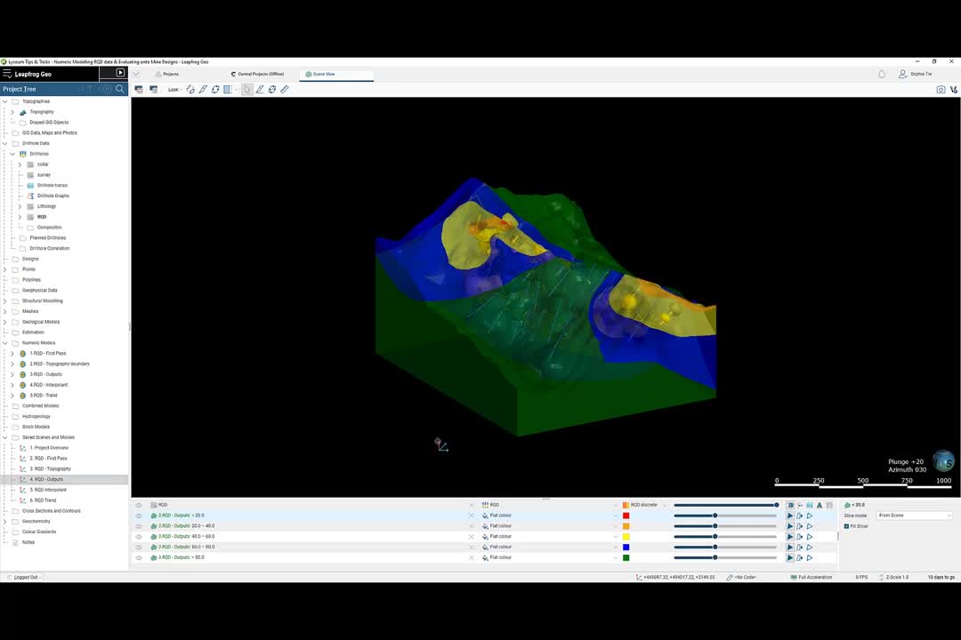
[00:05:46.950]And I’m going to type in values of 20, 40, 60, and 80

[00:05:53.750]for my new isosurfaces.

[00:05:57.550]I’ve also set my volumes to Enclose Intervals.

[00:06:01.618]In doing so, the interpolant

[00:06:02.930]will generate donut-shaped shells,

[00:06:04.670]in this case, the shells will be less than 20,

[00:06:07.630]20 to 40, 40 to 60, 60 to 80, and greater than 80.

[00:06:15.340]If I select higher values,

[00:06:16.750]the interpolant will generate a series of shells

[00:06:19.410]that enclose all higher values within them,

[00:06:21.760]in this case, greater than 20, greater than 40, and so on.

[00:06:25.900]And if I select lower values,

[00:06:27.717]the interpolant will generate a series of shells

[00:06:29.910]that enclose all lower values within them,

[00:06:32.000]in this case, less than 20, less than 40, and so on.

[00:06:38.650]Finally, the evaluation limits at the top here.

[00:06:44.000]The evaluation limits apply when interpolants

[00:06:46.270]are evaluated against other objects in the project.

[00:06:49.890]If we enable the evaluation limits,

[00:06:51.740]we would expect all values within the dataset

[00:06:55.780]that fall outside of the limits

[00:06:58.250]to be set to the minimum and maximum values here.

[00:07:08.810]We can now see that our model

[00:07:10.120]is starting to take better shape.

[00:07:16.620]The next settings I will look at are in the Interpolant Tab.

[00:07:20.050]Once again, I will double-click on the RQD model,

[00:07:22.390]but this time I will select the Interpolant tab.

[00:07:27.046]Understanding how the interpolation works is crucial.

[00:07:29.640]Leapfrog Geo can rapidly create models,

[00:07:31.470]however, they aren’t always correct.

[00:07:33.330]The default parameters will almost always be incorrect,

[00:07:35.530]so I’m going to run through a few rules of thumb

[00:07:37.520]that should work well

[00:07:38.400]for your geo-technical numerical models.

[00:07:40.910]The first thing we want to do

[00:07:41.890]is change the interpolant to spheroidal.

[00:07:48.100]By default, this is set to linear.

[00:07:52.430]Which will assume that values

[00:07:54.200]that are a certain distance from a particular point

[00:07:56.770]will have proportionately greater value on that point

[00:07:59.230]than values further away.

[00:08:01.180]By changing this to spheroidal,

[00:08:06.500]we will ensure that there is a finite point

[00:08:08.100]at which the influence of one point or another

[00:08:10.190]will fall to zero.

[00:08:11.860]Most geotechnical data will be better suited

[00:08:13.960]to a spheroidal interpolant.

[00:08:15.960]After a certain distance from an RQD point of, say, 20,

[00:08:19.440]we will reach a certain distance

[00:08:20.690]where this won’t have any effect on the RQD

[00:08:22.690]at another location.

[00:08:25.940]The total cell controls the upper limit

[00:08:29.020]of the interpolant functions,

[00:08:30.430]where there ceases to be any correlation between values.

[00:08:34.090]Closely spaced values are expected to be similar,

[00:08:36.600]and as the space between cells increases,

[00:08:39.230]their difference in value will too,

[00:08:40.760]until you reach the total cell

[00:08:42.110]where there will be no correlation between values at all.

[00:08:45.200]A good rule of thumb

[00:08:46.033]is to set this to the same as the variants.

[00:08:55.870]The base range is the parameter

[00:08:57.290]that corresponds to continuity.

[00:08:59.200]Increasing the base range will allow the isosurfaces

[00:09:01.800]to stretch a further distance between points.

[00:09:04.550]If the base range is set too small,

[00:09:06.100]the isosurfaces will not extend between your drillholes.

[00:09:09.360]As a rule of thumb,

[00:09:10.193]the base range can be set to around two to 2.5 times

[00:09:14.130]the average distance between drillholes.

[00:09:17.390]Currently the base range is set to 500.

[00:09:19.970]I’m going to change it to 600.

[00:09:28.810]Finally, the drift controls how the interpolant

[00:09:32.380]decays away from data.

[00:09:34.360]A drift of none will decay back to a value of zero,

[00:09:37.350]which we don’t want when we are interpolating RQD.

[00:09:40.580]And linear drift will decay linearly away from the data.

[00:09:45.180]And a constant drift means the interpolant

[00:09:47.060]will decay back to the mean of the data.

[00:09:49.700]This is the most appropriate option for geotechnical data.

[00:09:53.870]Don’t worry too much

[00:09:54.730]about the Alpha, Nugget, or Accuracy settings

[00:09:57.870]for geotech data.

[00:09:59.440]You can read up on these further in the online help manual,

[00:10:01.810]however, keeping them set to the default is generally fine.

[00:10:08.810]You can see the modifications I have made

[00:10:10.720]by changing these parameters.

[00:10:16.303]I’ll just quickly flip between the two.

[00:10:37.219]Okay.

[00:10:42.350]The final setting I would like to demonstrate

[00:10:44.100]is how to apply a trend,

[00:10:45.280]which you will already be familiar with

[00:10:46.690]if you have applied global trends to your geological models.

[00:10:49.870]Coming to the Trend tab of my editing window.

[00:10:56.930]You can see that I have applied a trend

[00:10:58.540]and the same orientation as a fault in my model.

[00:11:21.150]This fault is associated with low RQD values.

[00:11:24.530]To apply the orientation of this fault as a trend

[00:11:27.080]I have used the Plane tool in the toolbar

[00:11:31.020]to draw a plane in the scene.

[00:11:33.070]And then I have applied the orientation of this plane

[00:11:35.310]as my global trend.

[00:11:40.618]Here’s my plane which I have drawn.

[00:11:44.887]And the orientation can be changed

[00:11:47.390]by using these handles on the plane tool.

[00:11:53.690]I have then selected Set From Plane,

[00:11:57.300]which has applied the orientation of this plane

[00:11:59.170]as my global trend.

[00:12:12.270]Let’s take a look at my…

[00:12:22.090]So here is my final numeric model

[00:12:23.760]with a global trend applied.

[00:12:29.220]And as a comparison, here’s what it looked like

[00:12:32.860]when it did not have a trend applied.

[00:13:00.840]I will now quickly demonstrate

[00:13:02.160]how to evaluate a numeric model

[00:13:03.830]onto a mesh or development shape.

[00:13:19.950]As you can see,

[00:13:20.783]I’ve already evaluated my RQD model onto my pet mesh.

[00:13:28.240]To evaluate a numeric model onto a mesh,

[00:13:30.400]simply right-click on your mesh in the project tree

[00:13:33.030]and select Evaluations.

[00:13:36.490]Then select the numeric model

[00:13:38.010]you wish to evaluate onto that mesh

[00:13:39.990]by bringing it over to the selected column, and press OK.

[00:13:45.740]You can then bring your meshes into the scene

[00:13:47.750]if you have not already done so,

[00:13:49.700]and color by that evaluation.

[00:13:55.350]Just ensure you have applied the correct color gradients.

[00:14:01.550]That concludes this tips and tricks session

[00:14:03.480]on numeric modeling, geotechnical numeric data,

[00:14:07.150]and evaluating onto mine designs.

[00:14:10.380]There will be another session which will cover

[00:14:12.190]how to constrain numeric models using distance functions,

[00:14:15.180]and existing categorically modeled domains.

[00:14:21.470]If you’d like to know more about

[00:14:22.720]how the workflow as demonstrated in today’s webinar

[00:14:24.920]can add value to your project’s organization,

[00:14:27.190]feel free to get in touch using the contact details

[00:14:29.510]shown on screen.