Modeling with no drillholes (Remote Roundup 2021)

Leapfrog Geo allows you to easily construct geological models from any input data. In this demo, we’ll build a model from a geological map, some mapped surface contacts, and surface structural measurements.

Overview

Video Transcript

[00:00:01.487]
(upbeat music)

[00:00:10.520]
<v Anne>Thank you everyone for joining me today</v>

[00:00:14.940]
and taking time to join me for this webinar on creating

[00:00:19.090]
a geological model without drill holes in Leapfrog Geo.

[00:00:23.820]
My name is Anne Belanger

[00:00:25.140]
and I’m a project geologist at Sequent.

[00:00:27.940]
I’m based in Vancouver

[00:00:31.350]
and I’ve been with this team since March 2019.

[00:00:35.830]
We’re just going to get right into Leapfrog Geo.

[00:00:43.120]
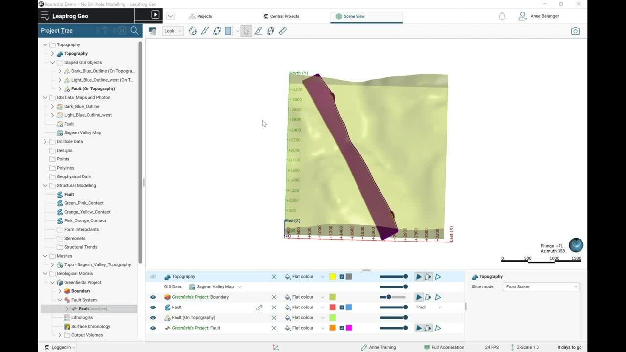
So we’re starting today’s demo with some pre-loaded data.

[00:00:47.360]
I have my topography, which was created from a mesh surface.

[00:00:53.950]
I have a geological map that was geo-referenced

[00:00:56.450]
and is now draped on the topography.

[00:00:59.720]
I have structural measurements that have been taken

[00:01:03.671]
at each contact sort of point or points

[00:01:07.230]
along each contact between these rock units.

[00:01:11.860]
And I also have some GIS lines

[00:01:16.330]
for my dark blue and light blue units.

[00:01:23.240]
So we’re starting off as mentioned.

[00:01:25.680]
We have no drill hole data, and we want to make a model

[00:01:30.960]
from this map using this information.

[00:01:35.160]
This scenario might arise maybe you’ve acquired a property

[00:01:38.950]
from either prospector or looking at some public access

[00:01:44.780]
geo-science data from local governments.

[00:01:48.680]
And also obviously the opportunity for companies

[00:01:53.270]
to do their own geological mapping campaigns.

[00:01:56.250]
And you want to analyze your information in a 3D format.

[00:02:02.000]
So I would like to start my model but first I do need

[00:02:06.090]
to capture all the data.

[00:02:08.960]
Or first I want to capture all the data

[00:02:10.480]
that is displayed here.

[00:02:12.170]
We have our contact information as mentioned,

[00:02:17.780]
in structural disks but I don’t have any information

[00:02:21.370]
for the fault yet.

[00:02:23.220]
So I’d like to digitize my fault

[00:02:25.780]
and then we can start our geological model.

[00:02:30.530]
So it’s easy enough to digitize the fault.

[00:02:34.160]
I’m just going to start by making a GIS line.

[00:02:39.440]
As with Leapfrog Geo and most sort of activities new icons

[00:02:44.780]
will appear in my toolbar that will allow me

[00:02:47.230]
to create this GIS line.

[00:02:54.570]
I can just trace it out to the best of my capabilities,

[00:03:05.900]
and end it by right clicking.

[00:03:09.470]
So easy enough I have my fault digitized

[00:03:12.380]
and just click Save.

[00:03:14.750]
This automatically creates a fault in my GIS data maps

[00:03:19.100]
and photos folder and also my fault draped on topography.

[00:03:28.170]
Next we can see that we have two structural measurements

[00:03:31.570]
taken along the fault.

[00:03:32.940]
They’re a little bit offset probably just because,

[00:03:38.090]
otherwise I wouldn’t be able to see the actual measurement.

[00:03:42.000]
So I would like to digitize these as well.

[00:03:43.780]
So someone was in the field and took a strike

[00:03:47.280]
for an azimuth strike dip of this fall.

[00:03:50.570]
To digitize the fault, structural measurements I can just go

[00:03:54.100]
to my structurally modeling folder and say new planar data

[00:03:58.940]
and also make sure that it is for my fault.

[00:04:08.740]
And to capture this information I just need

[00:04:11.230]
to create a structural disk.

[00:04:13.580]
I’ll make sure it’s on my fault.

[00:04:15.820]
So I just click and drag and try and align my azimuth

[00:04:19.860]
with the azimuth of the measurement on the map.

[00:04:24.570]
And I can type in my dip.

[00:04:26.520]
So 65, I could type in my azimuth if I knew

[00:04:32.180]
the exact measurement there, but instead I’ll just try

[00:04:35.300]
and match the alignment of my structural disk

[00:04:39.930]
with the measurement on the map.

[00:04:42.430]
I can type in 60, for my dip, and save.

[00:04:56.790]
So just easy as that, you know, we don’t need drill holes

[00:05:00.900]
we already have the information to build our fault

[00:05:03.720]
with the GIS line and our structural disk.

[00:05:09.720]
I can now create my geological model.

[00:05:15.300]
So I can just go to my geological model folders,

[00:05:17.320]
right click, a new geological model.

[00:05:22.930]
Surface resolution can be 50.

[00:05:25.070]
I want to make sure that my boundary

[00:05:28.877]
for my model only extends to the map.

[00:05:34.200]
Extends this way I’m not projecting my sort of calculations.

[00:05:42.750]
That’s where the map is and just make it

[00:05:45.180]
a little bit deeper at the end.

[00:05:48.020]
I’m going to name this green fields project.

[00:05:53.320]
And click okay.

[00:06:00.570]
We can see a processing as well, so often with Leapfrog Geo

[00:06:03.720]
when you are, when you create a new surface or add

[00:06:08.240]
some new information you will see the processing panel go.

[00:06:14.650]
For my geological model I have a boundary

[00:06:16.910]
which is now clipped by my topography.

[00:06:24.704]
And since we didn’t bring in drill holes I also,

[00:06:28.432]
so I have the startings of a geological model

[00:06:30.610]
but I don’t yet have my lithologies yet because

[00:06:33.240]
I didn’t create a base table for my geological model.

[00:06:36.680]
So I just in this particular case

[00:06:38.650]
I can enter in my lithologies manually.

[00:06:45.730]
We are going to just start by naming,

[00:06:49.456]
we’re just going to name them by their color.

[00:06:56.830]
Yellow, and I’m doing this in chronological order.

[00:07:05.410]
So I’ve gone from youngest to oldest.

[00:07:10.010]
Once again to help us model I am going to pick

[00:07:16.970]
this corresponding color for my corresponding unit.

[00:07:23.770]
I find it easiest at least in this particular case

[00:07:26.480]
to just click pink color.

[00:07:33.480]
And okay.

[00:07:40.520]
So now we have our framework for the model.

[00:07:44.964]
What we will be doing next is creating surfaces

[00:07:50.910]
that will be cutting into our boundary unit.

[00:07:56.250]
So we have this whole just massive volume per se

[00:08:02.060]
and if you can imagine that it’s like clay

[00:08:04.600]
and we’re going to just start cutting it up

[00:08:06.380]
into different lithological units and boundaries.

[00:08:12.360]
I’m going to start by actually splitting my model in two.

[00:08:20.050]
So I’m going to actually cut it by the fault which will

[00:08:22.380]
separate my models into an east and a west block.

[00:08:28.750]
So I’m just going to right click on fault system

[00:08:31.120]
and say new fault.

[00:08:33.810]
I did create my fault with both a GIS line.

[00:08:38.960]
I have information for both the GIS line

[00:08:40.850]
and structural disks.

[00:08:42.570]
I can start creating my folder with either option

[00:08:46.010]
but for now I’ll start with my structural disks.

[00:08:51.760]
Say okay.

[00:08:56.480]
And I’m just going to turn off exactly band

[00:08:59.530]
so we can see that fault a bit better.

[00:09:09.540]
So now we do have a line for our fault.

[00:09:15.010]
But as we can see it doesn’t quite follow the GIS line

[00:09:21.740]
because I haven’t yet told it to follow the GIS line.

[00:09:24.160]
So again, easy to create structural data

[00:09:27.200]
but also pretty easy to edit and adjust it.

[00:09:29.960]
So for this fault I can just right click on my fault line

[00:09:33.330]
and say add information and I’ll add my GIS line.

[00:09:39.610]
Make sure I pick my fault on topography,

[00:09:46.240]
and we can see that fault adjusts to typography.

[00:09:49.810]
So before it was just connecting the two structural disks

[00:09:53.080]
and now it follows the line that I traced on the map.

[00:10:00.770]
Again, as I mentioned we’re going to separate

[00:10:03.340]
this one model into two.

[00:10:05.340]
So I just want to activate my fault system.

[00:10:14.648]
I click okay, and we’ll see

[00:10:16.140]
in my project tree two fault blocks will appear.

[00:10:30.740]
So it’s now been cut by the fault

[00:10:32.180]
and we have two distinct blocks.

[00:10:40.990]
I activated my fault.

[00:10:43.030]
So my approach is to split this model.

[00:10:45.110]
I’m going to start by modeling my west block first

[00:10:50.040]
rather than my east block.

[00:10:51.320]
We can see the mythologies are quite similar in both

[00:10:54.384]
which will be beneficial for us and I can show.

[00:10:57.700]
Even though I’m starting with my west block I have

[00:10:59.390]
a little trick later on

[00:11:00.860]
to easily get my east block up to date.

[00:11:10.246]
I can figure out which block is which.

[00:11:12.410]
So my west block is my fault block two and my east block

[00:11:16.360]
is my fault block one.

[00:11:17.900]
So I want to start my modeling in this west block

[00:11:20.820]
which is my fault block two.

[00:11:29.350]
We have these four units

[00:11:31.640]
are green, pink, orange, and yellow.

[00:11:34.595]
I’m going to start by creating surfaces

[00:11:37.149]
for these four units.

[00:11:39.720]
As I mentioned previously we’re going to use these surfaces

[00:11:41.840]
to cut up this sort of boundary block.

[00:11:46.480]
And with four units we need three surfaces.

[00:11:50.760]
So I’m going to start with a deposit surface

[00:11:54.690]
and say new deposit from structural data.

[00:12:01.743]
I can tell Leapfrog Geo which unit is older

[00:12:05.040]
or younger than the other.

[00:12:06.270]
So in this particular case my pink is younger than my green.

[00:12:11.440]
And I’d like to use the pink

[00:12:14.795]
and green structural measurements

[00:12:18.330]
that my geologist made in the field.

[00:12:24.320]
So I dragged that surface in

[00:12:25.530]
and it is now cutting through this volume.

[00:12:31.920]
I can do this again for our orange to pink.

[00:12:34.680]
So new deposit from structural data, orange

[00:12:41.390]
is younger than pink.

[00:12:48.110]
Make sure to pick the proper measurements.

[00:12:56.293]
And once again we have a surface generated

[00:12:58.710]
along that contact point that cuts through our volume.

[00:13:03.750]
And so for the last one new deposit from structural data.

[00:13:09.270]
I’m going to do my yellow to orange contact and surface.

[00:13:25.670]
I can drag that in.

[00:13:28.300]
Drag the surface in and now we have all three surfaces

[00:13:32.871]
for all those units.

[00:13:35.860]
We’ll start right now by activating these surfaces

[00:13:38.370]
to create output volumes.

[00:13:41.310]
So right now our output volumes are unknown.

[00:13:44.300]
We don’t have any but once we activate

[00:13:46.300]
these surfaces same as our fault.

[00:13:48.841]
I just need to click the check mark and say okay

[00:13:52.560]
and make sure they were in chronological order

[00:13:54.470]
which they were.

[00:13:56.660]
And now we will see four different output volumes generated.

[00:14:09.437]
So to make it easier

[00:14:10.270]
to view these I’ll just drag them all in.

[00:14:15.245]
And there we go.

[00:14:16.840]
We have a piece of our initial block model.

[00:14:25.656]
And that looks pretty good to me.

[00:14:29.970]
I guess the only thing that we have to do now is look

[00:14:31.940]
at our blue units, so we have our blue on topography

[00:14:36.700]
and our light blue GIS lines.

[00:14:40.770]
We can see on the map there were no structural measurements

[00:14:42.362]
made at these contact points.

[00:14:45.830]
I guess also important

[00:14:46.840]
to be aware of what’s going on geologically.

[00:14:49.090]
So here we have a little bit of an angular unconformity.

[00:14:52.840]
So it looks like we have an original surface

[00:14:54.880]
maybe a little bit of geologically, you know,

[00:14:57.280]
a transgression regression cycle going on.

[00:15:00.490]
So in terms of this particular surface to create

[00:15:04.270]
for my blue units I’m going to use an erosional surface.

[00:15:12.170]
So I can start in my surface chronology

[00:15:13.990]
and say new erosion from GIS vector data.

[00:15:19.553]
And I can use just my GIS line that’s on the topography.

[00:15:25.970]
And I’ll pick my dark blue is younger than unknown.

[00:15:29.270]
For this particular case as well I’m going to stick

[00:15:31.750]
with my psychomythology being unknown

[00:15:34.080]
because my dark blue contacts multiple units I wanted

[00:15:38.250]
to take into account all those units rather than just one.

[00:15:42.390]
So I can say okay.

[00:15:50.084]
And we can see our surface is generating.

[00:16:01.230]
There we go.

[00:16:04.290]
So next I’d like to do my light blue as well.

[00:16:08.290]
So I’ll go with new erosion.

[00:16:10.930]
From new erosion, from GIS vector data

[00:16:22.670]
and I’ll pick that light blue.

[00:16:26.630]
And in this case I can say my light blue is younger

[00:16:29.260]
than my dark blue because my light blue unit

[00:16:32.100]
only touches my dark blue.

[00:16:34.820]
So I can say okay.

[00:16:44.570]
And I can drag my new surface into the scene as well.

[00:16:52.950]
So we can see we have these surfaces now

[00:16:55.060]
but we haven’t again activated them.

[00:16:57.280]
So Leapfrog Geo doesn’t know yet to create volumes

[00:16:59.610]
from them where to cut or other volumes by these surfaces.

[00:17:04.970]
Just need to double click on surface chronology and activate

[00:17:07.654]
these two surfaces and we’ll see these volumes adjust.

[00:17:16.930]
And we’ll also have two new volumes in our output volumes.

[00:17:21.070]
So we’ll get a dark blue and light blue volumes

[00:17:30.670]
and we’ll see the top of our other units disappear.

[00:17:34.410]
So now they have a flat cut off.

[00:17:39.380]
And if I just drag these two volumes in,

[00:17:53.460]
we now have our dark and light blue units.

[00:18:03.670]
Oh, if I look at my map again I can certainly see

[00:18:12.193]
that my west block is quite accurate.

[00:18:16.810]
So I’ve got my units all lining up and made

[00:18:23.350]
from depositional surfaces and then also erosions

[00:18:26.620]
for the blue units

[00:18:28.380]
which are just lying on top of our other lithologies.

[00:18:35.430]
So I’ve mapped the west side this west block now.

[00:18:40.950]
For our fall block one or east block we still

[00:18:44.760]
just have sort of blank data.

[00:18:48.320]
If you remember I mentioned a trick though.

[00:18:51.090]
So again, pretty lucky I can just go

[00:18:55.610]
to my surface chronology in the block I already modeled

[00:18:59.750]
and I can right click and say copy chronology two.

[00:19:05.810]
And it knows my only other block in this model

[00:19:09.160]
is my fault block one.

[00:19:10.940]
So I’ll click okay.

[00:19:13.784]
So what Leapfrog Geo doing now is it’s quickly

[00:19:15.710]
taking all those roles I just applied in my west block

[00:19:20.670]
and applying them to all those similar boundaries

[00:19:26.170]
in the east block.

[00:19:29.790]
So it’s going to take because we have

[00:19:31.700]
our structural information in both sides of the fault.

[00:19:36.640]
It can now create surfaces and output volumes

[00:19:42.000]
for this east side without me having

[00:19:45.230]
to go through and create all those rules again.

[00:19:52.520]
And there we go.

[00:19:55.300]
So it already brought it into the scene and if I just

[00:19:59.160]
turn my map back on and toggle

[00:20:02.270]
in between it looks pretty similar to me.

[00:20:07.760]
So that looks great.

[00:20:08.593]
We made our map, we made our model from our map.

[00:20:12.800]
So didn’t have any drill holes, it was nice and quick.

[00:20:18.510]
So I hope this helped provide some insight

[00:20:20.320]
into Leapfrog Geo’s capabilities.

[00:20:24.410]
Please feel free to ask questions now and type them

[00:20:26.860]
now we’ll continue to take them,

[00:20:29.570]
but that’s the end of the demo for now.

[00:20:32.240]
So Sarah, do we have any questions that came out?

[00:20:39.780]
<v Sarah>Hey, can you hear me okay?</v>

[00:20:41.840]
<v Anne>Yep.</v>

[00:20:43.170]
<v Sarah>Yeah, great thanks.</v>

[00:20:45.210]
Thanks for that demo.

[00:20:46.460]
I do have a few questions that popped up.

[00:20:48.630]
So first one is, if I had some downhaul structural data

[00:20:55.740]
obviously this was from some mapping but if I had some

[00:20:58.160]
from my drill called can I use it in a model in Leapfrog?

[00:21:02.040]
<v Anne>Yeah, yeah absolutely.</v>

[00:21:03.818]
So obviously, we don’t have draw holes in this model

[00:21:08.040]
to show but certainly when you have drill holes

[00:21:11.120]
in a project structural data can easily be brought in.

[00:21:14.430]
So added to the drill holes just by importing

[00:21:16.870]
the structural information to the drill holes folder.

[00:21:21.750]
These input like these inputs obviously need a depth.

[00:21:24.970]
So a depth at which they were taken in the drill hole

[00:21:27.360]
and then either a sorry, azimuth or dip or an alpha beta.

[00:21:32.226]
And from there you can view them in the draw holes

[00:21:34.430]
and also create syrinx from the information and obviously

[00:21:38.450]
just use it further for any structural calculations.

[00:21:42.610]
<v Sarah>Great, thanks for that.</v>

[00:21:45.764]
Another question, can you draw cross-sections as inputs?

[00:21:50.280]
So can you import cross-sections into Leapfrog and then use

[00:21:55.040]
that to add to your geological model in your interpretation?

[00:22:00.850]
<v Anne>Yeah and Sarah please feel free</v>

[00:22:02.450]
to add anything here.

[00:22:03.590]
So we can bring in import cross sections and view them

[00:22:07.100]
in our scene

[00:22:07.933]
when they’re sort of a geo-tiff and geo-referenced.

[00:22:10.880]
And then we could also trace those contact lines

[00:22:15.540]
within the sections to create those sort of GIS lines

[00:22:19.963]
that we created these surfaces from.

[00:22:22.760]
Sarah do you have anything to add for that?

[00:22:26.200]
<v Sarah>No that’s definitely true the other thing,</v>

[00:22:28.730]
the opposite of what you can do there

[00:22:30.320]
is actually create the cross sections within Leapfrog.

[00:22:33.210]
So if you’ve built a conceptual 3D model

[00:22:36.720]
like this we can then use Leapfrog to cut this model up.

[00:22:41.930]
Create the sections and then you can do

[00:22:43.820]
further interpretation work on that on paper

[00:22:46.060]
if you print them out or anything like that.

[00:22:47.760]
So it’s really easy to move between 2D and 3D space

[00:22:52.560]
in Leapfrog I suppose which is where I’m going with that.

[00:22:57.310]
No question.

[00:22:58.143]
Okay, one last question that’s popped up is,

[00:23:01.840]
how does Leapfrog calculate the offset along that fault.

[00:23:06.950]
<v Anne>Oh, that’s a good question.</v>

[00:23:09.960]
Leapfrog does not calculate the offset along the fault.

[00:23:13.750]
So when we activated the fault what we actually did

[00:23:17.013]
was told Leapfrog to disassociate essentially one side

[00:23:23.810]
from the other.

[00:23:24.643]
So instead of actually taking into account the fault

[00:23:27.670]
and instead just looks at the data on either side

[00:23:30.130]
of the fault completely separate from the other.

[00:23:33.010]
So I guess in this particular case

[00:23:35.820]
we had some good data capture in the field.

[00:23:39.400]
So we have some contact points, pretty close to our faults,

[00:23:44.340]
showing the sort of dip

[00:23:46.948]
or striking dip of those contact points as well.

[00:23:50.510]
And all that geo does is it takes that information.

[00:23:52.619]
So first on that west block it took all the information

[00:23:57.140]
and created our surfaces only with the input

[00:23:59.720]
in the west block, and then it did the same thing

[00:24:02.340]
for only the input on our east block.

[00:24:04.240]
So certainly, you know, it does our data capture

[00:24:10.060]
in this particular case was great.

[00:24:11.430]
So we are getting this sort of offshoot up top

[00:24:15.050]
into our model.

[00:24:16.620]
But yeah it actually doesn’t look at offset at all,

[00:24:21.470]
I guess if you were looking to know how much offset

[00:24:24.410]
there was in between the two fall blocks you could

[00:24:27.630]
as a rough tool just use a ruler to drag it out.

[00:24:32.510]
But yeah Leapfrog doesn’t actually look at that at all.

[00:24:37.770]
<v Sarah>Great.</v>

[00:24:39.230]
Okay and that’s all the questions that we’ve got for today.

[00:24:43.140]
So thanks for that.

[00:24:45.320]
And unless you’ve got anything to add

[00:24:46.820]
I think that’s it for this demonstration.

[00:24:51.560]
<v Anne>Nope, that’s it I guess like my email</v>

[00:24:53.360]
is just anne.belangerseequent.com.

[00:24:55.820]
If you have any questions I hope to talk to everyone soon.

[00:24:59.360]
Thanks for joining.

[00:25:02.402]
(upbeat music)