Mapping the groundwater systems of California with airborne geophysics

Over the past four years, Professor Knight and colleagues have explored using an airborne geophysical method to support groundwater management. Geophysical images have revealed the complexity of saltwater intrusion along the California coast, and the spatial variability in sediment texture in two parts of the Central Valley. About to be announced: a $12 million state-wide program to use the airborne geophysical method to map the groundwater basins of California.

Overview

Video Transcript

[00:00:15.550]
<v ->Hello, everybody.</v>

[00:00:16.550]
I am delighted to be here

[00:00:18.420]
talking about Mapping the Groundwater Systems of California

[00:00:21.340]
with Airborne Geophysics.

[00:00:24.120]
So, first of all, to introduce a simple schematic I use,

[00:00:26.830]
the tree is not to scale.

[00:00:28.540]
This is a slice through the subsurface

[00:00:30.700]
looking hundreds of meters below the ground surface.

[00:00:34.340]
And then to introduce my topic of interest, Groundwater.

[00:00:38.910]
The water that’s held in the openings

[00:00:40.770]
in the sediments and rocks below the ground surface.

[00:00:44.400]
Groundwater makes up 97%

[00:00:46.960]
of all the liquid freshwater on the planet,

[00:00:49.480]
so it’s essential to our groundwater supply,

[00:00:52.800]
both for people and for healthy ecosystems.

[00:00:56.320]
And so it’s essential

[00:00:57.330]
that we figure out ways to measure, monitor, manage

[00:01:01.770]
the quantity and quality of our groundwater resources.

[00:01:06.150]
So how do we get the information we need

[00:01:07.940]
about these groundwater systems?

[00:01:10.010]
One way is drilling, using wells.

[00:01:12.770]
And wells give us a great deal of information,

[00:01:14.930]
but only at the specific location where we have the well.

[00:01:17.640]
We don’t know what’s happening between the wells

[00:01:19.940]
or below the depth of the wells.

[00:01:22.500]
And so I have spent a lot of time

[00:01:24.990]
thinking about how to use imaging methods,

[00:01:27.680]
geophysical imaging methods,

[00:01:29.780]
to probe our groundwater systems.

[00:01:33.170]
And the method I’ve been working on

[00:01:34.640]
for the last several years

[00:01:35.890]
is the airborne electromagnetic method.

[00:01:38.720]
The airborne electromagnetic method

[00:01:40.410]
is a helicopter-deployed system.

[00:01:42.130]
The one we’re using is a helicopter-deployed system,

[00:01:44.220]
which moves the geophysical instruments

[00:01:46.430]
over the ground surface.

[00:01:47.870]
The instruments are held about 30 meters above the ground.

[00:01:51.050]
The system’s moving about 80 kilometers an hour,

[00:01:53.720]
so you can cover large areas in a day.

[00:01:57.080]
And we’re typically obtaining measurements

[00:01:59.740]
imaging to a depth

[00:02:00.900]
of about 300 meters below the ground surface in California.

[00:02:05.210]
So this then gives us a way

[00:02:07.150]
of getting the information we need

[00:02:08.730]
about our groundwater systems.

[00:02:12.590]
How does the EM method, electromagnetic method, work?

[00:02:15.900]
What we’re really mapping out

[00:02:17.160]
is the electrical resistivity of the subsurface.

[00:02:19.810]
So what we can derive from the acquired airborne EM method

[00:02:23.790]
is a model of the electrical resistivity of the sub-surface.

[00:02:28.170]
What we want to do with that model

[00:02:29.920]
is to recover the information about what’s truly down there.

[00:02:33.510]
So we want to take that electrical resistivity image

[00:02:37.450]
and transform it to map out the spatial variation

[00:02:41.710]
in the geologic materials that are holding our groundwater

[00:02:44.840]
to map out the spatial variation in lithology

[00:02:47.560]
or in sediment texture.

[00:02:49.360]
And we can also use the airborne EM method

[00:02:51.790]
to look at water quality issues, to map out salinity,

[00:02:55.210]
because all of these are sensitive,

[00:02:57.930]
or the electrical that we’re measuring,

[00:03:00.100]
is sensitive to all of these.

[00:03:03.840]
So I’m going to talk about, first of all, about an example

[00:03:06.650]
of using the airborne electromagnetic method

[00:03:09.200]
to obtain critical information

[00:03:11.580]
about the variation in water quality in an area.

[00:03:15.890]
And the study I’m going to describe

[00:03:17.940]
is one where we were looking at saltwater intrusion

[00:03:20.810]
along the Monterey coast.

[00:03:22.520]
So this is the central California coast

[00:03:25.280]
adjacent to Monterey Bay.

[00:03:27.370]
And this was a great project.

[00:03:29.210]
You can see the list of people involved here

[00:03:31.480]
and the funding sources.

[00:03:32.750]
And the study was recently published.

[00:03:35.260]
This image shows you immediately

[00:03:37.520]
why we have a problem with saltwater intrusion

[00:03:39.460]
along the Monterey coast.

[00:03:40.540]
Here’s extensive agriculture,

[00:03:42.420]
which is heavily dependent upon the pumping of groundwater.

[00:03:45.600]
And that pumping of groundwater

[00:03:47.260]
when you’re right next to the Pacific ocean

[00:03:49.760]
draws the Pacific Ocean into the groundwater aquifers.

[00:03:53.900]
So we get this seawater, this salt water,

[00:03:57.250]
intruding into our groundwater supply.

[00:04:02.610]
This is not just a problem along the California coast,

[00:04:06.060]
half the world’s population

[00:04:07.710]
lives within 60 kilometers of the coast,

[00:04:10.170]
groundwater provides the water supply,

[00:04:12.710]
and there is saltwater intrusion

[00:04:14.380]
occurring all over the world

[00:04:16.230]
as these coastal aquifers are pumped

[00:04:18.480]
to the extent that the ocean water is moving in.

[00:04:22.270]
And this is not just a problem

[00:04:23.810]
for the humans living along these coastal areas,

[00:04:26.910]
it’s also a problem in terms of the ecosystems.

[00:04:29.800]
Some of the richest ecosystems on the planet

[00:04:32.600]
are found within a kilometer of the coast.

[00:04:34.960]
So these coastal ecosystems depend upon this groundwater

[00:04:39.410]
moving out into the ocean to deliver nutrients.

[00:04:43.400]
Therefore, the moment we have saltwater intrusion,

[00:04:45.420]
we’re not only disrupting the human water supply,

[00:04:48.380]
but we’re disrupting the nutrient supply

[00:04:51.200]
to these coastal ecosystems.

[00:04:55.070]
Here’s a simple schematic of saltwater intrusion

[00:04:57.500]
along the Monterey coast.

[00:04:58.840]
There’s two levels from which water is being extracted,

[00:05:02.440]
an upper aquifer and a lower aquifer

[00:05:04.680]
separated by a clay layer.

[00:05:06.630]
And over time what’s happened is,

[00:05:08.680]
first of all, the shallow wells pumped extensively,

[00:05:11.780]
so saltwater moved into the upper aquifer.

[00:05:14.320]
And then the wells went into the deeper zone

[00:05:16.570]
and saltwater moved into the lower aquifer.

[00:05:19.700]
And what’s needed along this coast,

[00:05:21.950]
the groundwater managers who are trying to grapple

[00:05:24.400]
with this problem, in order to undertake

[00:05:26.960]
any sort of proactive groundwater management,

[00:05:29.240]
they need to know

[00:05:30.073]
where is the salt water, fresh water interface.

[00:05:34.090]
So we use the airborne EM method

[00:05:36.470]
to look at answering that question.

[00:05:39.420]
There was information from WellData,

[00:05:41.367]
but it just didn’t provide the kind of spatial density

[00:05:45.550]
that was really needed

[00:05:46.680]
to understand what was happening there.

[00:05:49.140]
So here’s the airborne EM system

[00:05:50.850]
being put together at a local air field.

[00:05:53.470]
This is the big transmitter loop

[00:05:55.630]
with the receiver at the back of the transmitter loop.

[00:05:58.360]
The helicopter comes in, lifts it up

[00:06:01.410]
and flies out across the study area.

[00:06:06.140]
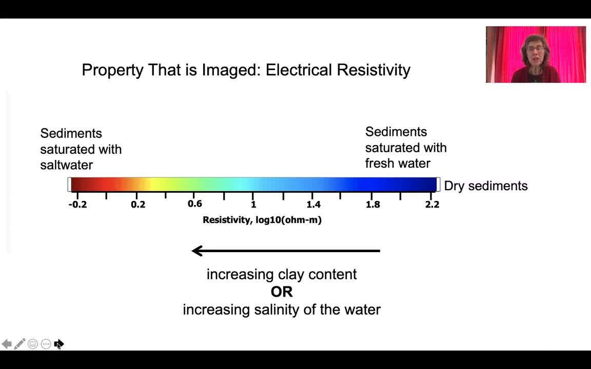
So what’s being mapped, as I mentioned,

[00:06:07.860]
is electrical resistivity.

[00:06:09.300]
So in this study, what we’re doing is mapping out

[00:06:12.340]
the color scale here I’m showing.

[00:06:14.550]
Blue are the sediment saturated with fresh water.

[00:06:17.400]
Dark blue are very dry sediments at the ground surface,

[00:06:21.240]
so they’re very resistive.

[00:06:22.620]
And then red, so low electrical resistivity.

[00:06:26.350]
Red is where we have salt water.

[00:06:28.690]
The sediments, the aquifer now

[00:06:30.790]
has been filled with salt water.

[00:06:32.470]
So, simple color scheme.

[00:06:34.260]
Blue is good, it’s fresh water.

[00:06:35.900]
Red is bad, it’s salt water.

[00:06:39.810]
Now, in between,

[00:06:41.070]
the reason we’re not interpreting that region in between is,

[00:06:43.930]
it definitely gets more complicated.

[00:06:46.190]
Your resistivity could be changing

[00:06:47.840]
because of a change in the composition of the sediments.

[00:06:50.800]
There’s more clay there

[00:06:52.210]
that tends to have low electrical resistivity,

[00:06:54.910]
or it could be due to a change in salinity.

[00:06:57.250]
So we really can’t separate these two factors.

[00:07:00.220]
So what we do is;

[00:07:01.550]
blue is freshwater,

[00:07:02.990]
red, low resistivity, is saltwater.

[00:07:07.350]
And here’s the starting point for this survey.

[00:07:09.260]
We had this image along the coast

[00:07:11.290]
acquired using another form of geophysical data,

[00:07:14.420]
where we saw the red, salt water, and the blue, fresh water.

[00:07:18.010]
And that contour that you’re seeing

[00:07:19.860]
is the interpretation based on wells

[00:07:22.180]
as to the extent of the saltwater.

[00:07:24.910]
All those dots that are appearing

[00:07:27.020]
are where we acquired our airborne EM data.

[00:07:29.710]
So you can see that continuous flight lines.

[00:07:33.170]
The colors that are appearing

[00:07:35.240]
indicates blue where we have fresh water,

[00:07:38.260]
red where we have saltwater.

[00:07:39.500]
And this is an absolutely phenomenal dataset.

[00:07:43.770]
When the water managers in the area saw this,

[00:07:46.100]
they were absolutely amazed.

[00:07:47.050]
Here’s red, the salt water that we have all along the coast,

[00:07:51.120]
and then moving inland,

[00:07:52.660]
definitely a more complicated situation,

[00:07:55.230]
but you could never resolve this by drilling wells.

[00:07:58.520]
But with this density of data,

[00:07:59.950]
you can start to see what’s happening.

[00:08:01.920]
You can start to see what’s controlling

[00:08:04.050]
the saltwater intrusion.

[00:08:06.350]
And so we can take data such as this,

[00:08:09.100]
come up with a slice through our data

[00:08:11.950]
and look what’s happening as we’re moving to the north.

[00:08:14.130]
Now, what you’re seeing here is this classic image

[00:08:16.660]
of a saltwater intrusion wedge.

[00:08:18.490]
This wedge of salt water with the overlying freshwater.

[00:08:22.950]
And as we go to the north,

[00:08:24.360]
you see a much more complicated pattern

[00:08:26.500]
with the red saltwater extending inland

[00:08:29.020]
in places where the salt water

[00:08:30.550]
is getting into the underlying region.

[00:08:33.470]
So a data set like this is absolutely invaluable

[00:08:37.610]
for groundwater management in coastal areas

[00:08:39.670]
and being able to visualize it like this,

[00:08:41.870]
using Leapfrog to display this

[00:08:44.620]
complicated spatial density of data

[00:08:48.020]
and interact with groundwater managers and hydrologists.

[00:08:51.370]
It’s just been phenomenal for looking at this problem

[00:08:55.070]
in this area.

[00:08:57.490]
So the next thing I want to talk about

[00:08:59.010]
is thinking about groundwater quantity.

[00:09:01.670]
And thinking about groundwater quantity,

[00:09:03.700]
we don’t directly detect groundwater quantity

[00:09:07.090]
with the airborne EM method.

[00:09:08.700]
But what we do is map out the sediment types

[00:09:11.970]
in the subsurface.

[00:09:13.280]
And we map out where we have sands and gravels

[00:09:16.230]
that hold and move large volumes of water.

[00:09:19.270]
And we map out where we have clays that can hold water,

[00:09:22.880]
but act as impediments to flow.

[00:09:24.640]
And you can’t pump water out of clay.

[00:09:26.430]
So mapping out what’s down there in terms of the composition

[00:09:29.950]
is an essential part of managing groundwater quantity.

[00:09:34.540]
So I’m going to put my quantity story

[00:09:37.090]
in the context of a much larger project.

[00:09:39.690]
This is a project funded at Stanford

[00:09:41.480]
by the Moore Foundation;

[00:09:43.060]
Advancing Earth Imaging Technologies

[00:09:45.110]
to Reveal the Scale-Dependent Dynamic

[00:09:47.460]
of Groundwater Systems.

[00:09:48.680]
And I have a short movie to show you just as an example,

[00:09:52.000]
all the different data sets we’re pulling together;

[00:09:54.380]
satellite data, ground-based data,

[00:09:56.240]
of course, our airborne electromagnetic data,

[00:09:58.830]
and data that we’re just pulling in from various sources,

[00:10:02.660]
snow water equivalent data,

[00:10:04.840]
looking at reservoir storage data,

[00:10:07.280]
looking at InSAR data,

[00:10:08.760]
which maps out defamation of the ground surface here

[00:10:12.490]
due to groundwater extraction,

[00:10:15.000]
and then our airborne EM data.

[00:10:17.580]
The team of people at Stanford listed at the top,

[00:10:20.070]
and the movie you’re about to see

[00:10:21.350]
was put together by Seogi Kang at Stanford using Leapfrog.

[00:10:27.400]
So, you’re going to be looking

[00:10:28.500]
at the Central Valley of California shown here.

[00:10:31.800]
All the green, it’s an agricultural area,

[00:10:34.600]
but in terms of climate, very close to a desert.

[00:10:38.130]
And so, understanding groundwater quantity here,

[00:10:41.420]
thinking about groundwater management here,

[00:10:44.000]
we pull together various data sets,

[00:10:46.420]
all of which are part of understanding

[00:10:48.750]
the delicate balance in this area

[00:10:50.890]
in terms of groundwater quantity,

[00:10:52.880]
because groundwater is being extensively pumped

[00:10:55.730]
to support irrigation.

[00:10:57.990]
So the starting point shown here as snow water equivalent

[00:11:02.790]
is the snowpack that’s accumulating in the Sierras

[00:11:06.210]
over the winter months.

[00:11:07.600]
And even though there’s rain in the valley itself,

[00:11:11.440]
it’s the snow pack that accumulates over the winter

[00:11:14.950]
and then melts in the spring and moves down into the valley

[00:11:18.870]
that is really essential for supporting irrigation.

[00:11:23.410]
And what you start to see, there’s going to be the rivers,

[00:11:26.560]
and then there’s a system of canals

[00:11:28.120]
moving the surface water around.

[00:11:30.500]
And the reservoirs that you’ll see as white dots

[00:11:33.850]
that are sized based on the amount of water stored

[00:11:37.940]
in those reservoirs,

[00:11:39.300]
quite variable between the Southern part

[00:11:41.630]
of the Central Valley and the Northern part.

[00:11:44.190]
Definitely more water in the north.

[00:11:46.400]
And what that means is limited water supply,

[00:11:49.470]
limited surface water supply in the south,

[00:11:51.900]
so extensive of groundwater, which results in,

[00:11:55.280]
up comes our interferometric synthetic aperture radar data.

[00:11:58.210]
We’re looking at the subsidence in red.

[00:12:00.830]
These are parts of the ground that are sinking

[00:12:03.460]
because of over pumping of the groundwater.

[00:12:06.550]
What you’re seeing here is the total subsidence

[00:12:08.880]
between January, 2015 and September, 2019,

[00:12:13.740]
and the maximum subsidence 1.3 meters.

[00:12:16.720]
So just over that four years, 1.3 meters.

[00:12:20.240]
So we went in with our airborne EM

[00:12:22.390]
to help groundwater managers understand

[00:12:24.870]
what was controlling the quantity of groundwater,

[00:12:27.650]
where is their groundwater in this area,

[00:12:30.260]
what could be done thinking strategically

[00:12:33.210]
about where to pump and how to pump.

[00:12:35.610]
And what I’m showing now, the data being filtered

[00:12:38.880]
just to show where there’s a lot of clay-rich materials

[00:12:41.810]
in the subsurface.

[00:12:43.120]
‘Cause definitely, if you’re extracting water

[00:12:45.640]
and there’s a lot of clay present,

[00:12:47.190]
it’s the compaction of these clays

[00:12:49.290]
that causes the subsidence.

[00:12:51.560]
So data such as this, images such as these,

[00:12:54.900]
help ground water managers think strategically

[00:12:57.300]
about where to pump, how much to pump

[00:13:00.310]
and also think strategically about opportunities

[00:13:03.090]
for getting water back into the subsurface.

[00:13:06.230]
And coming up now,

[00:13:07.480]
just focusing at the detail of what’s happening

[00:13:10.820]
at the interface between the Sierra Foothills

[00:13:13.800]
and the Central Valley,

[00:13:15.430]
we’re going to be doing some more flying

[00:13:17.470]
along that exact interface

[00:13:20.600]
to really understand how recharge from the Sierras

[00:13:23.480]
is getting into the Central Valley.

[00:13:27.170]
So, I hope I’ve convinced you,

[00:13:29.120]
airborne EM is a way of answering these questions

[00:13:32.450]
that are important about water quantity and water quality,

[00:13:35.530]
or a way of getting the data we need

[00:13:37.660]
to start managing, measuring

[00:13:39.840]
and monitoring groundwater quantity and quality.

[00:13:43.330]
And this has become really urgent now in California.

[00:13:47.690]
In 2014, with the passage

[00:13:49.460]
of the Sustainable Groundwater Management Act, which says,

[00:13:52.727]
“All of the groundwater in California,” thankfully,

[00:13:56.627]
“now needs to be sustainably managed.”

[00:13:59.470]
And groundwater management plans are due 2020,

[00:14:03.280]
so some were due this year, and 2022.

[00:14:06.180]
So there is an urgent need for water agencies

[00:14:09.240]
to figure out what is happening below the ground surface

[00:14:12.950]
in terms of ground water quantity and quality.

[00:14:16.680]
Well, I’m delighted to say that in 2019,

[00:14:19.240]
there was the passage of proposition 68,

[00:14:21.680]
and it means that the Department of Water Resources

[00:14:24.060]
has committed $12 million to using this airborne EM method

[00:14:29.790]
to map out the subsurface

[00:14:31.870]
in groundwater basins of California.

[00:14:34.080]
And what that’s done is raised this question,

[00:14:36.720]
how do we do this throughout California?

[00:14:39.670]
So for the past two years, I’ve been leading

[00:14:41.800]
what’s known as the Groundwater Architecture Project.

[00:14:45.010]
And it was a pilot study working in three areas to say,

[00:14:49.010]
what is the optimal workflow for acquiring airborne EM data?

[00:14:53.270]
All the people involved shown here

[00:14:55.710]
and the locations of where we were working shown here;

[00:14:59.570]
Butte County, San Luis Obispo County, Indian Wells valley,

[00:15:03.710]
our funding sources.

[00:15:05.440]
And I encourage you to look at our website,

[00:15:07.415]
mapwater.stanford.edu,

[00:15:10.500]
where we go through this whole workflow

[00:15:14.300]
for acquisition of airborne EM data

[00:15:16.300]
under what I call this decision-aware geophysics umbrella,

[00:15:20.280]
where we’re constantly focused on:

[00:15:23.240]
What are the questions we’re asking?

[00:15:25.150]
What are the groundwater management decisions

[00:15:27.370]
that need to be addressed?

[00:15:31.140]
And so I’ll zoom in one more time

[00:15:32.980]
showing the airborne EM data from Butte County.

[00:15:35.810]
This was a phenomenal data set.

[00:15:37.750]
And here the warm colors are mapping out

[00:15:40.640]
where there are sands and gravels, where there’s clay.

[00:15:44.040]
And so data such as this,

[00:15:46.230]
these types of images are just so essential

[00:15:51.360]
for starting to manage groundwater in an area.

[00:15:55.640]
So I’ve talked a lot about California,

[00:15:58.020]
but I just want to leave you with the message

[00:16:02.160]
that this isn’t just a California problem,

[00:16:04.430]
groundwater resources around the world are being challenged

[00:16:08.590]
because of climate change,

[00:16:09.910]
because of a population that is on its way

[00:16:12.540]
to 10 billion people.

[00:16:15.320]
And I believe that those of us who have the knowledge

[00:16:18.470]
to address these global problems should be doing so.

[00:16:21.330]
It’s not just,

[00:16:22.510]
an incredible opportunity with this knowledge

[00:16:24.680]
comes an opportunity to work on these amazing problems,

[00:16:28.450]
but with knowledge also comes a responsibility

[00:16:31.620]
to do what we can to address these global problems.

[00:16:35.590]
And I believe, in terms of addressing the global issue

[00:16:39.560]
of managing, protecting our groundwater resources,

[00:16:43.630]
I believe geophysics has an important role to play.

[00:16:47.410]
And I see my role as helping to ensure that that happens.

[00:16:52.210]
Thanks very much.