Leapfrog Works – Building a 3D Geologic Model of an Earthen Dam Site

Leapfrog Works helps you visualise and understand your data so you can communicate risks with stakeholders of all technical levels – and make better decisions on all your civil engineering and environmental projects.

In this webinar, we will:

• Explore the Leapfrog Works interface
• Import an array of data types (including imports from Central Seequent’s cloud-based model management solution)
• Build a geological model utilizing drilling data
• Quickly validate a first pass build of a geologic model
• Quantify lithologic volumes
• Generate cross sections along an alignment
• Export compatible data types to be used in programs such as GeoStudio

Presenter: Sean Buchanan – Project Geologist, Denver, CO
Sean Buchanan is a Professional Geologist with a BSc in Geology from the University of North Carolina Wilmington.
Sean spent two years as a wellsite geologist in the Permian Basin before joining AECOM. While in consulting, Sean supported a large-scale hydrogeologic characterization at an active coal-burning power generation facility, as well as a handful of chlorinated solvent sites.

Sean is currently a Project Geologist at Seequent, where he works closely with business, sales, marketing, and technical teams to provide high quality solutions for geoscience professionals.

Overview

Video Transcript

[00:00:00.733]
(soft music)

[00:00:10.680]
<v Sean>Hi guys, and welcome to today’s webinar</v>

[00:00:12.940]
on building 3D geological models within Leapfrog Works.

[00:00:16.580]
My name is Sean Buchanan,

[00:00:17.730]
a project geologists out of Denver, Colorado.

[00:00:20.980]
Today we’re going to be building an earthen dam

[00:00:22.810]
or embankment dam site, mainly utilizing drilling data.

[00:00:28.540]
Here’s a look at our agenda for today.

[00:00:30.910]
So first I’ll be briefly discussing

[00:00:32.960]
the Leapfrog Works interface to get you oriented.

[00:00:36.210]
I’ll then introduce the sites

[00:00:37.880]
and completed first pass model,

[00:00:39.750]
so you can see what we’ll be building today.

[00:00:42.380]
I’ll then start a brand new project and start importing data

[00:00:46.610]
from local files as well as Central,

[00:00:49.380]
which is sequence cloud based model management solution.

[00:00:53.720]
We’ll then get into building out our geological model,

[00:00:56.430]
utilizing an array of geologic surface types.

[00:00:59.910]
After that model is complete,

[00:01:01.880]
we will do some model validation

[00:01:04.270]
and check our model against our borings.

[00:01:07.720]
Finally, we will generate cross sections along an alignment

[00:01:10.760]
and look at some of those data output types.

[00:01:13.640]
So this is a lot really trying to give you as much exposure

[00:01:16.690]
as possible looking into Leapfrog.

[00:01:20.830]
So after that, we will finish with a live Q and A,

[00:01:24.540]
but please feel free to ask any questions

[00:01:27.630]
during the webinar.

[00:01:28.463]
We’ll either address them then and there,

[00:01:30.740]
or we’ll bring them to the live Q and A to talk about.

[00:01:34.370]
So thanks again for joining

[00:01:35.630]
and we’ll go ahead and get started.

[00:01:39.430]
This is the Leapfrog Works interface.

[00:01:41.810]
On the left-hand side, we have our project tree

[00:01:44.417]
and this is where all of our data lives.

[00:01:47.030]
The right click is very powerful in Leapfrog,

[00:01:49.410]
so if you want to import data,

[00:01:51.010]
you can just right click on one of these folders,

[00:01:53.140]
it will give you an array of data types to choose from.

[00:01:56.550]
This was built in a workflow oriented design.

[00:02:00.260]
So at the top, we can see we have topography, GIS data,

[00:02:03.850]
boreholes, followed by design files and so on and so forth.

[00:02:08.670]
In the middle of our project tree,

[00:02:10.340]
we have some of our model functionality,

[00:02:12.470]
so we can create geologic numeric or combined models.

[00:02:16.000]
At the bottom is some of our recording features.

[00:02:18.560]
So creating safe scenes in movies,

[00:02:20.890]
or cross sections in contours.

[00:02:23.520]
To the right of this project tree we have our scene view.

[00:02:28.010]
So I could pull over any data from my project tree

[00:02:31.130]
and view that in the scene.

[00:02:35.330]
So I just pulled in my boring data.

[00:02:38.660]
I can make this a little easier to view

[00:02:40.730]
by changing my Z scale.

[00:02:42.080]
So I can go to the bottom right-hand corner,

[00:02:44.290]
change my Z scale vertical exaggeration to two.

[00:02:49.750]
Underneath my scene view, I have my shapes list.

[00:02:53.630]
Whatever’s in my scene view is going to be populated,

[00:02:56.360]
in my shapes list as well.

[00:03:00.130]
There’s more functionality here

[00:03:01.690]
so I can turn things on or off, change the transparency.

[00:03:06.130]
I can change the width of my boreholes,

[00:03:10.540]
change the colors of certain attributes.

[00:03:14.440]
To the right of this,

[00:03:15.400]
I’m going to have a small properties panel.

[00:03:18.380]
So whatever I click on in my shapes list

[00:03:21.170]
is going to give me some new functionality down here.

[00:03:24.080]
So if I had a query filter, I can add those,

[00:03:27.040]
change the line radius.

[00:03:29.130]
These will all be different

[00:03:32.050]
depending on what object is in the scene.

[00:03:33.840]
So I can see my topo has some different customization tools

[00:03:40.090]
than my borehole file does.

[00:03:43.730]
At the top of my screen I have a toolbar

[00:03:47.020]
which has some pretty handy functionality.

[00:03:49.660]
I do have a ruler, so I can measure between borings.

[00:03:55.880]
I have a plane tool, so I can create planes,

[00:03:59.330]
which is really handy in the modeling process,

[00:04:01.570]
which I will show off later.

[00:04:05.450]
And we also have a slicer tool.

[00:04:07.860]
So this allows you to slice through your model

[00:04:13.770]
to do some data validation.

[00:04:17.130]
We also have a split screen view.

[00:04:19.570]
So I’ll just go ahead and put a new view up,

[00:04:22.130]
and this is my current transect line.

[00:04:25.120]
I can work through my model by clicking the period

[00:04:27.990]
or the comma sign.

[00:04:29.900]
So I’ll move south so I can see my transect,

[00:04:33.260]
transect is moving south,

[00:04:37.740]
and see how my model changes.

[00:04:44.050]
I then have some hotkeys here.

[00:04:46.360]
So if you want to look down on your model,

[00:04:48.460]
you can go here, press D.

[00:04:51.980]
It also tells you your hotkeys over here.

[00:04:54.100]
So I could just press D on my keypad.

[00:04:56.480]
I could press E to look east,

[00:05:01.210]
and so on and so forth.

[00:05:02.770]
I’m going to go ahead and clear my scene here

[00:05:04.490]
with this trashcan.

[00:05:06.170]
Great thing about Leapfrog is you never need to save,

[00:05:09.140]
it saves automatically for you.

[00:05:10.900]
So I’m just going to clear my scene

[00:05:12.660]
and introduce this project.

[00:05:16.260]
Let’s go and take a look at our final project

[00:05:18.510]
so we can see what we’re going to be doing today.

[00:05:21.440]
Once again, this is an earthen dam,

[00:05:23.260]
also known as an embankment dam.

[00:05:25.730]
These are mainly utilized for flood risk management,

[00:05:28.520]
water supply, and conservation,

[00:05:30.080]
as well as a variety of recreational purposes.

[00:05:32.770]
So here I have some topographic contours,

[00:05:35.710]
so we can understand kind of the lay of the site.

[00:05:38.130]
So our high points over here in the Northeast,

[00:05:41.510]
we also have this dam access line,

[00:05:44.190]
which we’ll be utilizing later to build cross sections

[00:05:46.740]
along that alignment.

[00:05:50.920]
The geology is mainly composed of glacial outwash deposits

[00:05:54.870]
of variable thickness as well as a few volcanic flows.

[00:05:58.910]
So the model is underlain by a basalt flow here in green.

[00:06:02.430]
And then we also have a more felsic volcanic flow

[00:06:05.320]
with this QPVD unit.

[00:06:08.780]
We’re going to build a first pass geological model,

[00:06:11.800]
utilizing this borehole data.

[00:06:14.100]
So we’re going to go through and build individual surfaces

[00:06:16.960]
for each of these units, starting with our basalt

[00:06:20.370]
and moving up into our sedimentary units,

[00:06:24.330]
and then into our outwash deposits.

[00:06:28.270]
We have a little bit of QAO maps at the site.

[00:06:31.490]
And then finally we will finish with our fill material.

[00:06:38.350]
Once the model is built,

[00:06:39.400]
we’re going to do some model validation.

[00:06:41.750]
So I’ll just cut a cross section

[00:06:43.380]
through the middle of this, kind of zoom in

[00:06:47.180]
and change the transparency of our output volumes.

[00:06:51.750]
And from here, we can work our way through our model

[00:06:55.490]
and see how our boreholes are being honored by our model.

[00:07:07.340]
After that, we’re going to build some cross sections

[00:07:10.430]
along this alignment.

[00:07:11.430]
So I’ll just go and push these into the scene.

[00:07:22.610]
So here we have some cross sections

[00:07:27.770]
that can either be pushed right into a report

[00:07:30.890]
or exported to a geo-technical software like GeoStudio

[00:07:35.400]
for further analysis.

[00:07:41.720]
So let’s go ahead, I’m going to clear the scene

[00:07:43.640]
and we’re going to start a new project

[00:07:45.510]
and import all of this data from Central.

[00:07:50.020]
So I’ve created a new project

[00:07:51.600]
within my Central Project Server.

[00:07:53.470]
Let’s called this name demo server.

[00:07:56.630]
For those who don’t know,

[00:07:57.960]
Central is sequence cloud-based model management solution,

[00:08:01.240]
designed for project teams managing complex geologic data.

[00:08:05.180]
So it’s a data management solution that helps visualize,

[00:08:07.760]
track and manage your geoscience data from a centralized

[00:08:11.120]
and auditable environment.

[00:08:13.220]
So that’s a great way to keeping project teams connected,

[00:08:16.400]
organized, and working in a version controlled space.

[00:08:20.990]
So basically once our model is complete,

[00:08:22.920]
we can publish that into Central.

[00:08:25.400]
So publish it into the cloud

[00:08:27.200]
where that data can be managed appropriately.

[00:08:30.180]
We’ll also be notified of any changes made to the model,

[00:08:34.270]
so we’re up to date with the latest developments

[00:08:36.140]
in your project.

[00:08:37.700]
We can also use web visualization,

[00:08:39.910]
so we can look at these models on the web to comment,

[00:08:46.840]
review, and manage shared ideas.

[00:08:50.840]
So let’s go ahead and go to our Central portal.

[00:08:54.160]
So I’ma hit these three dots and go to the portal.

[00:09:01.220]
And I’m not going to go into too much detail about Central.

[00:09:03.880]
We do have a lot of great resources online,

[00:09:06.830]
if you want to schedule a demo

[00:09:08.690]
or look into some of our training, we offer that.

[00:09:13.240]
So these are all of the projects within my Central server.

[00:09:18.180]
I’m going to go ahead and just search for the earthen dam.

[00:09:22.540]
This is blank right now, since I did erase everything

[00:09:26.230]
’cause we’re going to be starting from scratch.

[00:09:31.380]
Within my overview tab, I can see what’s been published

[00:09:34.600]
into my earthen dam project.

[00:09:36.630]
So I see I have a master branch

[00:09:38.870]
that was published by Peter in May, 2020.

[00:09:43.310]
Looks like Gary came in here

[00:09:44.157]
and tried to do some experimental phase

[00:09:46.280]
dam modeling in June.

[00:09:48.490]
And then today I’ve actually uploaded a blank project

[00:09:51.700]
’cause we’re going to be building this from scratch together.

[00:09:54.330]
What’s nice about this is I can click

[00:09:55.980]
on one of these published artifacts

[00:10:01.785]
and that’ll bring me to web visualization

[00:10:03.770]
where I can pull some of this data into the scene to view.

[00:10:06.930]
So just bring in my topography and maybe my drilling data.

[00:10:13.230]
So I can zoom in and look at some of this data.

[00:10:17.110]
Additionally, you do have some nice functionality.

[00:10:19.370]
You can change the Z scale if you need,

[00:10:24.520]
and cut transect lines, use the ruler,

[00:10:27.360]
very similar to Leapfrog Works.

[00:10:30.090]
What’s also great is we can add comments

[00:10:33.090]
to whatever we’re looking at in the scene

[00:10:34.610]
to collaborate around our models.

[00:10:36.150]
So if I wanted to leave a comment for someone,

[00:10:38.690]
I can just click on this message bubble.

[00:10:42.166]
I actually did this, I guess 55 minutes ago.

[00:10:45.940]
I left a comment for Stephanie asking,

[00:10:48.037]
“Please take a look at this possible drilling location.”

[00:10:51.060]
So I left this comment and I can actually click on this

[00:10:56.410]
and go exactly to where I left this comment,

[00:10:58.440]
which in this case is kind of an arbitrary location,

[00:11:03.640]
but Stephanie is able to respond,

[00:11:05.690]
go exactly to that comment to see what I was looking at.

[00:11:08.940]
And she was also, she would’ve gotten a notification,

[00:11:12.700]
in this notification bell up here,

[00:11:15.770]
so great way to communicate around our model.

[00:11:18.980]
So I’m going to go back into my main screen here.

[00:11:22.850]
I have this user’s tab.

[00:11:26.360]
This is where we have the option

[00:11:28.120]
of three different types of permissions.

[00:11:30.140]
You can be a viewer, an editor, or an owner.

[00:11:33.590]
An editor is someone who’s going to be going in

[00:11:35.730]
and making changes to the model,

[00:11:37.820]
but doesn’t have the permissions to add users

[00:11:40.650]
to this user base.

[00:11:42.420]
The owner is the only one who has the permissions

[00:11:45.260]
to add additional users.

[00:11:47.270]
And then a viewer is really only going to have access

[00:11:49.640]
to looking at these web visualizations.

[00:11:55.900]
We have this files tab, we call this the data room.

[00:11:58.610]
This is where you bring in all your project data,

[00:12:01.100]
and you can bring in data

[00:12:04.000]
directly from Central into your project.

[00:12:06.440]
What’s nice about that is you’ll get an icon

[00:12:09.810]
on your project,

[00:12:11.400]
for instance, if this borehole data gets updated,

[00:12:14.440]
there’ll be an icon on your project that’ll say,

[00:12:17.960]
basically your project data is out of date

[00:12:21.040]
and you can reload that to refresh your model.

[00:12:24.710]
We have a history tab,

[00:12:27.520]
which kind of looks like my overview tab,

[00:12:29.200]
but you can go in and change around, edit this history.

[00:12:32.520]
So if you want to change this model branch

[00:12:34.830]
or changing the name of it, you can do that here.

[00:12:37.800]
We have a scene tab for creating safe scenes.

[00:12:40.780]
So you can rapidly go in and fly to this exact scene

[00:12:44.790]
to look at web, in web visualization.

[00:12:48.070]
And then finally we have this events tab,

[00:12:50.690]
which is a full audit record

[00:12:52.310]
of what’s happened within your model.

[00:12:54.750]
So what users have been granted access,

[00:12:57.200]
who’s downloaded the model, who’s uploaded the model,

[00:13:00.130]
what comments have been made.

[00:13:02.020]
So here’s Stephanie just responded to my comment about,

[00:13:07.870]
maybe we take a look at the color data,

[00:13:09.700]
it looks like it may be off.

[00:13:14.320]
So that’s a very quick tutorial to Central,

[00:13:17.850]
but we’ll go ahead and start building our project out

[00:13:19.610]
for time sake.

[00:13:20.990]
So let me get out of my Central portal,

[00:13:23.930]
and I can actually go see this audit history as well,

[00:13:28.110]
of my project by going into my projects tab,

[00:13:31.820]
and I can actually search for my project here

[00:13:39.540]
within our projects tab.

[00:13:40.700]
So I have this earthen dam, so I can double click this.

[00:13:44.486]
And this brings me to an area

[00:13:46.180]
where I can download previous versions

[00:13:48.170]
or the most recent version of the model.

[00:13:52.350]
So let’s go back into our scene view

[00:13:54.090]
and we’ll start bringing in some of our project data

[00:13:56.770]
from Central.

[00:13:58.290]
So I’m going to go ahead and clear my scene.

[00:14:01.990]
Let’s go ahead and start importing some of our project data.

[00:14:04.700]
So we’re going to start with our topography surface,

[00:14:07.580]
but we’re actually going to bring that in

[00:14:08.500]
through our meshes folder first.

[00:14:10.470]
So I’m going to right click on meshes.

[00:14:13.170]
If we have this file locally, we can import mesh here.

[00:14:17.590]
For this case, we’re going to use Central to import this data.

[00:14:20.480]
So I’m going to select this second option.

[00:14:25.640]
We need to then find our earthen dam project,

[00:14:31.800]
and we can bring in data from previously published projects.

[00:14:36.420]
So if I did want to bring in this data

[00:14:38.170]
from our experimental branch,

[00:14:39.850]
I can just bring that in from here,

[00:14:41.690]
or we can go directly into the data room.

[00:14:44.760]
So I’m going to go ahead and select our files tab.

[00:14:47.890]
I’m going to go down to my topography,

[00:14:50.640]
and select this topography DXF.

[00:14:53.400]
At the bottom here, we can see our supported file formats.

[00:14:57.530]
So let me go ahead and bring this in.

[00:15:00.330]
And this is going to process,

[00:15:02.290]
so you can just click on your processing panel

[00:15:04.040]
and see how that’s doing.

[00:15:07.290]
I will say that sometimes if you bring in data

[00:15:10.670]
and it doesn’t seem to be processing, it may be paused.

[00:15:13.480]
So go ahead and click on your processing panel

[00:15:15.990]
and select the run all.

[00:15:17.740]
So that is processed, I can bring this into the scene.

[00:15:22.170]
That’s my topography mesh.

[00:15:25.130]
I can change the color of this if I wanted.

[00:15:29.880]
Now let me add this in the mesh.

[00:15:30.900]
We can actually add this to our topography file.

[00:15:33.890]
So I’m going to right click on topography.

[00:15:39.410]
And select new topography from surface,

[00:15:45.120]
and I can select this DXF file.

[00:15:52.890]
So that will process.

[00:15:54.580]
And now we have our topography surface.

[00:15:58.490]
We can go ahead and change this to an elevation color map.

[00:16:03.800]
Turn on the legend.

[00:16:06.660]
Something else I can do here is extract the vertices

[00:16:09.560]
that make up this surface.

[00:16:11.040]
To do that, I can right click topography

[00:16:13.420]
and select extract vertices.

[00:16:17.640]
Press okay, and that will populate my points folder

[00:16:22.210]
with these vertices.

[00:16:23.510]
I think this was initially a 10 foot lidar-DEM surface.

[00:16:32.520]
So I just imported just one file from Central.

[00:16:36.650]
Just wanted to give you guys a taste of what that’s like,

[00:16:39.440]
and the rest of this,

[00:16:40.530]
I’ll just be uploading data from my local drive.

[00:16:43.720]
So I have a folder with a few different types of data types,

[00:16:47.440]
some aerial images, GIS data, borehole data.

[00:16:50.650]
So we’ll go through that process now.

[00:16:53.730]
So let’s go ahead and bring in some GIS data.

[00:16:56.340]
So I’m going to right click GIS data, maps and photos,

[00:16:59.020]
select import map, and then I’ll grab my aerial image,

[00:17:06.890]
which is already geo-referenced.

[00:17:08.100]
We actually have the ability to geo-reference images

[00:17:11.780]
in Leapfrog, so definitely check out our website

[00:17:14.290]
for details on that.

[00:17:16.500]
So I can bring this into the scene

[00:17:19.640]
and then I’ll go ahead and bring in my dam access line.

[00:17:24.170]
So I’ll just import vector data here,

[00:17:27.960]
navigate to my access line

[00:17:35.120]
and also bring this into the scene.

[00:17:39.384]
And we can see this is kind of floating

[00:17:40.540]
above the surface currently.

[00:17:45.150]
So it’s actually below our topography surface,

[00:17:48.700]
it’s because we need to drape this on topography.

[00:17:51.440]
So I’m going to clear my scene.

[00:17:52.800]
Once again, I’m hitting the trashcan.

[00:17:54.720]
So I’ll bring in my topography surface.

[00:17:56.610]
I’m just going to change this to a flat color,

[00:18:01.270]
and underneath our topography in our shapes lists,

[00:18:04.420]
we have this GIS data dropdown.

[00:18:06.500]
So I’m going to go ahead and select this down arrow,

[00:18:09.880]
go to views and select edit views.

[00:18:15.780]
From here, I can create a new view.

[00:18:20.270]
I’ll call this ariel and access line.

[00:18:26.800]
This is going to let me move over my GIS data

[00:18:31.440]
to drape on topography.

[00:18:35.690]
You can change the line width.

[00:18:38.970]
So I’ll just go and change this to we’ll say eight

[00:18:42.220]
and I’ll make it red.

[00:18:45.200]
Also notice this is, this dam access line is above my ariel.

[00:18:50.600]
If it’s below this layer, it’s not going to be shown.

[00:18:53.840]
So make sure any of your line work

[00:18:56.170]
is on top of your aerial image.

[00:18:59.410]
And then let’s go ahead and press close.

[00:19:02.440]
And now that has draped on my topographic surface.

[00:19:08.680]
So I can make multiple views if I have a lot of GIS data,

[00:19:11.310]
I can just keep going in, go back into edit views,

[00:19:15.300]
create a new one.

[00:19:16.830]
I can also just show one GIS object at a time.

[00:19:20.920]
So if I wanted to go to do that, I can go to GIS objects

[00:19:23.900]
and select this dam access line, which will be shown there,

[00:19:27.080]
but I’d recommend creating a lot of views for easy access

[00:19:31.650]
to getting a better picture of your model.

[00:19:34.860]
Now that we have our GIS data,

[00:19:36.070]
let’s go ahead and import some of our borehole data.

[00:19:38.280]
So I’m going to right click the borehole data folder.

[00:19:41.950]
We have quite a few sources of data inputs here,

[00:19:44.950]
so I can bring in data via local CSV files.

[00:19:49.650]
We can import these via Central or in ODBC like gINT,

[00:19:54.040]
or Microsoft Access.

[00:19:56.440]
We can also, we have direct API with OpenGround cloud,

[00:19:59.760]
which is Bentley’s cloud-based geo-technical

[00:20:03.860]
data management platform.

[00:20:05.290]
So within OpenGround,

[00:20:06.370]
you can create boring logs, cross sections.

[00:20:09.750]
There’s quite a bit of recording functionality in there,

[00:20:12.670]
so this API will continue to get better.

[00:20:16.040]
And then we can also add core photo links.

[00:20:19.730]
So this would be like connecting

[00:20:20.840]
to something like a (indistinct).

[00:20:23.720]
So we are actually just going to use CSV files.

[00:20:25.780]
I’m going to import here and now I can go ahead

[00:20:29.290]
and navigate to my color file.

[00:20:32.320]
I’ll select this color.

[00:20:34.290]
That’s actually going to auto map my survey files,

[00:20:36.230]
since it had survey in the file name,

[00:20:39.800]
and now I need to go import my geology table,

[00:20:43.620]
which has my interval data.

[00:20:45.200]
If I have, say I have another interval table,

[00:20:48.670]
like RQD data or some sort of downhole CPD measurements,

[00:20:53.760]
I can also bring those in.

[00:20:55.180]
I’ll just have to add that plus sign.

[00:20:57.210]
If you have any numeric data

[00:20:59.210]
or maybe some downhole point data, bring those in here.

[00:21:02.410]
And if you’re using the hydrogeo extension,

[00:21:05.470]
you’ll be able to import your screen intervals.

[00:21:09.300]
So this is all I have for this site, actually.

[00:21:11.540]
So I’ll just go and press import.

[00:21:16.560]
And depending on what your headers are,

[00:21:18.248]
this may auto map automatically

[00:21:21.440]
for what type of data this is.

[00:21:23.890]
So this actually auto mapped all this for me,

[00:21:26.870]
since my CSV file had a hole ID, an X, Y Z,

[00:21:32.090]
as well as a max depth.

[00:21:33.788]
So it’s quite handy to have a max depth in your color file

[00:21:36.960]
because Leapfrog does an automatic QA/QC

[00:21:40.450]
when you import this data.

[00:21:41.690]
So for instance, if you have a geology interval

[00:21:45.440]
that exceeds your max depth of say a hundred,

[00:21:48.140]
it’s going to flag that as an error.

[00:21:50.670]
So let’s go and press next.

[00:21:52.270]
We can see I’m on my survey table now.

[00:21:55.340]
If you’re working on a site with all vertical holes,

[00:21:58.360]
you don’t need this survey table.

[00:21:59.920]
I think there is some dip in some of these holes.

[00:22:01.670]
So I have one here with hole ID, depth, depth,

[00:22:05.670]
and my azimuth.

[00:22:08.210]
If one of these aren’t mapped or mapped incorrectly,

[00:22:10.600]
you can always go in and change these

[00:22:12.400]
to whatever type of data it is.

[00:22:14.810]
So I’m going to go and click next.

[00:22:19.440]
So here, once again hole ID, I’ll have my from two interval

[00:22:22.850]
and now I have a couple lithology codes.

[00:22:25.240]
So it actually did map these.

[00:22:26.800]
So I’m going to go and click this header,

[00:22:29.000]
and I’m going to bring this in as geology.

[00:22:32.470]
And same thing here, I do have some rippability versus fill,

[00:22:35.970]
so I can bring this in.

[00:22:37.690]
I can bring it as lithology if I wanted,

[00:22:39.670]
or a category if you had say, whoever logged the hole

[00:22:44.600]
or a drill rig, you can bring those in as categories.

[00:22:47.210]
We have timestamps data or dates,

[00:22:51.080]
obviously map it correctly.

[00:22:54.690]
So I’m going to go ahead and press finish.

[00:22:58.650]
That is going to process.

[00:23:07.250]
Oops, looks like we already had some in here.

[00:23:08.780]
I’m just going to go ahead and delete my first borehole set

[00:23:13.280]
and rename this.

[00:23:20.520]
So now I can bring in my geology into the scene.

[00:23:24.780]
I can see that I have a, I do have an error here.

[00:23:29.630]
So I have this red exclamation point,

[00:23:32.160]
so I can go ahead and right click on this

[00:23:34.440]
and navigate to those errors so I can select fixed errors.

[00:23:40.130]
So this is part of that QA/QC process.

[00:23:42.340]
So I can investigate these

[00:23:44.040]
and I can see that I have some hole IDs

[00:23:46.380]
that are not in my color table.

[00:23:48.800]
So these are in my interval table, but not in my color,

[00:23:51.270]
so obviously, I don’t have a location for them.

[00:23:54.900]
I have some warnings where I also have no color,

[00:23:57.710]
no samples for my color.

[00:24:02.880]
So nothing I really need to do here.

[00:24:05.876]
But if I did want to fix these errors,

[00:24:07.140]
I mean this was a tall tale sign

[00:24:09.630]
I’m missing some survey data.

[00:24:11.770]
So you’d want to export these errors out

[00:24:14.680]
depending on what they are,

[00:24:15.700]
get them to your database manager to fix in your raw data,

[00:24:19.210]
because you can fix these in Leapfrog,

[00:24:21.120]
but we don’t recommend doing that.

[00:24:22.830]
We always recommend fixing your original data source.

[00:24:29.280]
So here are my borings with my drilling code.

[00:24:34.427]
I’m going to go ahead and change my Z scale

[00:24:36.600]
so we can see these a little better.

[00:24:38.840]
And also I can import, I have a Leapfrog color file

[00:24:42.020]
for these lithology types,

[00:24:44.950]
I want to be consistent in my recording

[00:24:46.540]
and use the same colors, so I can go ahead and import these.

[00:24:49.786]
I’m just going to right click on my grouped code,

[00:24:52.900]
go to my colors and select import.

[00:24:59.050]
So I’m going to go back a few, I do have this grouped code,

[00:25:02.280]
and let’s see Leapfrog color file.

[00:25:07.860]
Oops, Imported on the wrong one.

[00:25:11.120]
So we’ll go in here, try that again.

[00:25:16.710]
So there we go, some consistent colors

[00:25:19.370]
with my previous projects.

[00:25:21.200]
So there we go, finally we’ve got our data imported,

[00:25:25.000]
and now we can start building this model.

[00:25:29.250]
A few last words before you start your model.

[00:25:31.680]
It’s a great idea to really understand your data

[00:25:33.860]
the best you can, do you want to look for trends?

[00:25:36.150]
You really want to understand your geologic history.

[00:25:38.420]
It’s only going to help your modeling process in the end.

[00:25:41.140]
So you can do that by looking at each unit individually.

[00:25:45.950]
So I’m going to flick on one unit at a time,

[00:25:48.730]
and you can see some of the space

[00:25:51.900]
and geographic relationships between these.

[00:25:54.050]
So I’ve got my fill, my QAL kind of over on this east side.

[00:26:03.190]
Some of the sedimentary units seem to be stacked up nicely,

[00:26:07.270]
kind of around the entire site.

[00:26:12.136]
I do have a felsic volcanic unit over on the east side

[00:26:15.310]
of this dam as well.

[00:26:18.630]
Slope wash, another sedimentary unit,

[00:26:22.730]
and then my basalt at the bottom of my model.

[00:26:27.050]
So definitely something to keep in mind

[00:26:28.790]
before you start.

[00:26:33.650]
To create a geological model,

[00:26:35.250]
we’re going to right click on our folder

[00:26:36.960]
and select new geological model.

[00:26:40.550]
From here, we can choose the base lithology column.

[00:26:43.140]
So this is what we’re going to build our services from.

[00:26:45.600]
This is our, we’re going to choose our DH code.

[00:26:48.410]
Something to note,

[00:26:49.243]
you can only choose this this base lithology column once.

[00:26:52.950]
So definitely choose the right column to model from.

[00:26:56.300]
Our surface resolution I’m going to set at 25.

[00:27:00.110]
And this is important because it controls how fine

[00:27:03.000]
or coarse the surfaces, so the lower surface resolution,

[00:27:06.890]
the smaller the triangles are,

[00:27:08.427]
and the more definition the surface will have.

[00:27:11.410]
The higher the resolution,

[00:27:14.480]
the less time it will take to process,

[00:27:16.240]
but may not show the level of detail that you might want.

[00:27:18.470]
So it really depends on the type of detail you want,

[00:27:20.990]
how big your project is.

[00:27:23.780]
Finally, we can move into our boundary model extent box.

[00:27:27.900]
So we can see we have these toggles in the scene.

[00:27:30.070]
So I can change this box using these arrows.

[00:27:34.130]
I can also type in these values manually,

[00:27:36.980]
or I can enclose the model on an object,

[00:27:41.540]
which is pretty handy.

[00:27:42.760]
I’m going to go ahead and choose that,

[00:27:44.150]
enclose it on my lithology data.

[00:27:47.700]
So it’s going to retrofit my model boundary

[00:27:49.810]
to only include areas where I have drilling data.

[00:27:56.120]
So I’m just going to call this earthen dam GM,

[00:28:01.510]
and I’ll press okay.

[00:28:05.180]
Under our new earthen dam GM,

[00:28:07.580]
we can see we have some new folders down here.

[00:28:10.070]
So the first one being our boundary folder,

[00:28:12.770]
this is basically just a blank model

[00:28:16.160]
of our geologic boundary, so I can actually click on this,

[00:28:20.330]
it’s going to show me the volume and the area.

[00:28:25.460]
So what’s going to happen is we’re going to parse

[00:28:26.980]
this boundary up into different geologic units

[00:28:30.980]
to create a airtight geological model.

[00:28:33.950]
Under our boundary, we have our fault system.

[00:28:36.490]
We’re not going to be mapping any faults in this webinar,

[00:28:38.660]
but if you did have them,

[00:28:39.670]
that’s where you’re going to have them.

[00:28:41.280]
We have a lithologies folder,

[00:28:43.080]
and then maybe the two most important

[00:28:44.770]
in the modeling building process is the surface chronology

[00:28:48.690]
in the output volumes.

[00:28:50.360]
So our surface chronology is where we’re going to build

[00:28:53.790]
our individual surfaces using an array of surface types.

[00:28:57.220]
So deposits, erosions, intrusions, veins, and so on.

[00:29:01.370]
And once we build those surfaces and activate them,

[00:29:04.440]
we will be given these output volumes

[00:29:07.300]
of each of our surfaces.

[00:29:09.030]
So right now we just have this unknown,

[00:29:11.870]
which is once again, basically just our model boundary.

[00:29:17.210]
So let’s go ahead and create our first surface type.

[00:29:20.730]
So I’m going to go ahead and bring my geology

[00:29:22.460]
back in the scene.

[00:29:25.700]
Now I can go ahead and start building my geological model.

[00:29:28.680]
So I’m actually going to go into my lithology legend,

[00:29:31.960]
which can be turned on or off from here,

[00:29:33.880]
and change the order of these

[00:29:35.140]
to the units that I’ll be building first.

[00:29:37.540]
So I’m going to start with my slope wash unit,

[00:29:39.460]
and then move into my felsic volcanic rock.

[00:29:43.190]
And then I’ve got my fill, my recent alluvium or QAL.

[00:29:47.350]
I’ve got an older slope wash units, a fluvial,

[00:29:49.750]
a (indistinct) and undifferentiated sedimentary deposits,

[00:29:53.660]
and then finally I’ll finish with my tertiary basalt.

[00:29:56.620]
So I’ll press OK, and then I’ll reorder my legend.

[00:29:59.580]
To create a new surface, I’m going to go into my GM

[00:30:02.540]
and right click on surface chronology.

[00:30:05.180]
From here I can choose an array of surface types.

[00:30:08.890]
For the slope wash, I’m actually going to use an intrusion,

[00:30:11.210]
it’s kind of a irregular shape,

[00:30:13.250]
and I’m going to choose my base lithology, which is my DH code.

[00:30:17.070]
It’s what I’ve used for my earthen dam model.

[00:30:20.650]
And you can see we also have a few other types

[00:30:23.950]
of data we can use, so if we have other contacts,

[00:30:28.070]
polylines, points, services, that type of data,

[00:30:31.660]
we can use those as well.

[00:30:33.530]
So I’m going to go and select from base lithology.

[00:30:37.220]
My interior lithology is going to be this QSW,

[00:30:40.380]
and exterior is going to be all of my other units

[00:30:42.890]
that have not been modeled yet.

[00:30:44.560]
So I’ma go ahead and press okay, and that is going to process.

[00:30:50.405]
I’m just going to go ahead and turn everything off but my QSW,

[00:30:52.480]
just so we can take a look.

[00:30:56.250]
And I’ll pull this surface contact into the scene.

[00:31:01.040]
So like I said, this is somewhat irregular.

[00:31:03.820]
We can go in and set a trend,

[00:31:06.120]
a global trend to this to clean it up,

[00:31:08.390]
but for sake of time, which we are running out of,

[00:31:10.690]
I’m going to keep moving on just so you guys get exposed

[00:31:12.900]
to as much as possible.

[00:31:14.400]
So I’m going to build my next unit,

[00:31:16.220]
which is going to be also on the east side of my dam,

[00:31:21.060]
this felsic volcanic so I can look at that.

[00:31:26.160]
In the scene here I’ll have a few data points,

[00:31:27.710]
but it’s kind of in a similar trend,

[00:31:29.510]
kind of trending in this direction.

[00:31:31.380]
So to build that, once again I’m going to right click

[00:31:33.730]
on surface chronology,

[00:31:35.520]
I’m going to select new intrusion from base lithology,

[00:31:39.742]
and now I’m going to go ahead and select my QPVD unit.

[00:31:43.740]
And I’m going to move over my slope wash,

[00:31:46.340]
since I’ve already modeled those contacts,

[00:31:48.070]
I do not need to model them again.

[00:31:50.352]
So I’m going to go ahead and press okay and let that run.

[00:31:56.550]
And let’s bring this into the scene and see how it looks.

[00:32:00.430]
So it looks okay.

[00:32:01.950]
Something which you may notice is

[00:32:04.490]
there’s somewhat of a trend with this data,

[00:32:06.440]
as well as our last QSW data.

[00:32:09.060]
Only over here on the right side of our model

[00:32:12.170]
and some somewhat of a trend in this direction.

[00:32:14.400]
So something like this, you may want to set a global trend

[00:32:18.410]
to better inform your model.

[00:32:20.270]
To do that, the easiest way is to go up into this tool bar

[00:32:24.080]
at the top and select this draw plane line button.

[00:32:28.190]
From here we’ll just go and draw planes.

[00:32:31.640]
So I’m going to left click on my mouse, drag and kind of,

[00:32:36.290]
yeah, basically connect all these points together.

[00:32:38.860]
That’s going to create this plane,

[00:32:40.077]
and from here, I can go ahead and adjust this plane,

[00:32:42.330]
using these arrow toggles.

[00:32:45.510]
I can also go down here into my properties panel

[00:32:49.390]
and type these in manually.

[00:32:52.300]
So I think this direction looks pretty good.

[00:32:59.759]
And then we see we have this pitch currently at 176.

[00:33:02.980]
This pitch is actually going to be our line

[00:33:05.030]
of maximum continuity,

[00:33:06.430]
which can be changed by moving this green arrow.

[00:33:09.600]
So what this is going to do once we set this trend,

[00:33:12.390]
it’s actually going to stretch our interpolation

[00:33:15.350]
in the direction of this green arrow,

[00:33:17.970]
as well as our intermediate line,

[00:33:22.280]
which is always perpendicular to this,

[00:33:24.660]
as well as our minimum line, which is orthogonal to those,

[00:33:28.420]
so it’s actually in the Z direction.

[00:33:30.980]
So let me go into my trend tab to set this.

[00:33:33.740]
So I’m going to double click on my QPVD unit.

[00:33:39.010]
I’m going to go into my trends tab,

[00:33:42.390]
this is where we set this global trend,

[00:33:44.850]
and we can see we’ve already created this plane

[00:33:46.870]
in the scene, I can copy these attributes

[00:33:49.970]
or these numbers over to this by selecting set from plane.

[00:33:56.220]
So I’m just going to set from plane

[00:33:58.670]
and that’s going to match whatever was down here

[00:34:00.930]
in my properties panel into my direction.

[00:34:03.060]
And this has changed my ellipsoid ratio.

[00:34:05.990]
So before this is set at one, one and one,

[00:34:09.600]
which is a isotropic surface,

[00:34:12.110]
so equally weighted on all sides.

[00:34:14.850]
Now we’ve actually made this an isotropic,

[00:34:18.060]
because we are extending this,

[00:34:20.420]
we’re stretching this three times,

[00:34:21.640]
in our maximum continuity direction,

[00:34:23.720]
three in our intermediate,

[00:34:26.110]
and then one that’s actually staying the same.

[00:34:29.030]
So I’m just going to go on press okay and see how this changes.

[00:34:40.080]
So it looks a little better I’d say, I’m actually going to,

[00:34:44.360]
let’s go ahead and change these line radius

[00:34:48.380]
to a little thinner and I’ll get rid of my plane.

[00:34:53.270]
So that’s okay, this is kind of the iterative process.

[00:34:57.020]
If you want to go in and keep adjusting these ratios, you can.

[00:35:03.130]
So for instance, I can actually stretch this five times

[00:35:06.380]
in our maximum direction, see how that looks.

[00:35:11.220]
That looks a little better.

[00:35:13.100]
And then we can also make other explicit changes

[00:35:16.300]
within here, so I’m just going to press D on my keypad.

[00:35:19.200]
It looks like it’s blowing out a little bit over here.

[00:35:21.070]
I don’t have data, so I’m just going to go ahead

[00:35:23.770]
and right-click on my QPVD, and I can say select this edit,

[00:35:29.099]
and I can just edit with a polyline.

[00:35:32.280]
I’m sorry guys I’m flying through this,

[00:35:33.610]
we’re running out of time, but I can go ahead

[00:35:35.900]
and draw a polyline directly on this new surface.

[00:35:39.520]
So for instance, I can just, I’ll just draw a polyline,

[00:35:44.470]
something like this, and I’m going to go ahead and press save.

[00:35:50.820]
And this is going to reprocess this surface.

[00:35:53.330]
So it’s kind of sliced some of that off,

[00:35:54.840]
it looks a little better,

[00:35:56.640]
and I’ll just go ahead and get out of this toolbar

[00:35:58.370]
by pressing the X.

[00:36:00.720]
So now I have this polyline informing this surface.

[00:36:08.500]
Let’s continue to move on with our next surface,

[00:36:12.470]
which is actually going to be my fill.

[00:36:14.410]
So I’m going to go ahead and only show my fill contacts

[00:36:17.710]
in the scene, see what those look like.

[00:36:21.453]
I’ma go ahead and get rid of this polyline

[00:36:23.680]
as well as our QPVD.

[00:36:29.210]
Let’s go ahead and take a look at

[00:36:30.750]
where these fill contacts live geographically.

[00:36:33.310]
So I can go ahead and throw my topo in the scene,

[00:36:35.543]
just to get an idea, it seemed to run parallel

[00:36:39.220]
to our dam access line.

[00:36:44.150]
And we already have this surface built.

[00:36:45.690]
Actually it was built in Leapfrog

[00:36:47.930]
and those vertices were exported.

[00:36:51.910]
So I’m going to use that file to build the surface.

[00:36:54.970]
So I’m going to into my points folder,

[00:36:57.130]
and I’m going to right click and select import points.

[00:37:01.770]
And here I have this fill contact vertices.

[00:37:06.760]
So this is going to want me to map these data points,

[00:37:10.150]
so I just have an X, Y, Z, let’s map those correctly,

[00:37:12.930]
and select finish, and if I bring these into the scene,

[00:37:17.070]
it’s basically just a bunch of points.

[00:37:21.740]
That is going to be my contact surface.

[00:37:23.920]
So to build a new contact here,

[00:37:26.040]
I’m just going to right click on surface chronology.

[00:37:28.617]
I’m going to create this as an erosional deposit

[00:37:31.625]
and I’m going to use my points,

[00:37:32.865]
so I’m going to select from points.

[00:37:38.240]
From here, we’ll go ahead and select

[00:37:40.000]
our fill contact vertices.

[00:37:42.390]
We’ll select our fill for our first lithology,

[00:37:45.897]
and we will say that is younger than our second lithology,

[00:37:49.030]
which is unknown,

[00:37:50.670]
since we see that we are going to be contacting multiple units,

[00:37:56.630]
we can’t assign a single contact.

[00:37:58.670]
So we’re going to leave this as unknown

[00:38:01.090]
and I’ll go and press okay and let that process,

[00:38:04.180]
which may take a few minutes.

[00:38:05.880]
We do have quite a bit of data points here.

[00:38:09.080]
So we’ll go ahead and keep letting that run.

[00:38:14.150]
So our feel surface has processed.

[00:38:16.560]
Once again, this is an erosional surface

[00:38:18.350]
built with extracted vertices, this looks pretty good.

[00:38:22.230]
You may want to go in and add some additional polylines

[00:38:24.900]
to constrain this a bit,

[00:38:27.110]
but for now this will work just fine.

[00:38:29.120]
So now I want to build my next surface, which is this QAL.

[00:38:33.770]
So if I pinpoint this data in the scene,

[00:38:38.270]
I can see that it does have some variability

[00:38:41.010]
in the Z direction,

[00:38:42.260]
which may look like it could build a pretty irregular shape.

[00:38:47.700]
We don’t have many data points for it.

[00:38:49.270]
So I may choose to build this with a intrusive surface,

[00:38:54.860]
and I know this isn’t an intrusive body,

[00:38:56.710]
but there is a lot of functionality

[00:38:59.030]
with our intrusion surface type.

[00:39:04.050]
So let’s go ahead and give this a try.

[00:39:05.440]
So new intrusion from base lithology.

[00:39:10.270]
My interior lithology is going to be QAL,

[00:39:13.570]
and I want to ignore my field contact points

[00:39:18.120]
as well as my felsic volcanic,

[00:39:20.610]
as well as my upper slope wash.

[00:39:22.660]
I’ve already modeled these contacts,

[00:39:23.830]
don’t need to model them again.

[00:39:28.450]
So bringing this into the scene.

[00:39:33.390]
Doesn’t look great starting off,

[00:39:35.180]
so we may want to set a global trend.

[00:39:38.670]
You don’t really see a good trend,

[00:39:40.820]
I mean, maybe something like this.

[00:39:44.280]
Something you can also do instead of creating

[00:39:46.490]
an actual polyline is going into your trends tab.

[00:39:53.210]
So I haven’t built a plane yet, but I can view a plane,

[00:39:56.180]
which is just going to be basically a flat plane,

[00:40:00.870]
runs in the vicinity of our data.

[00:40:08.040]
So I don’t really see a clear trend with this.

[00:40:10.410]
So I’m going to leave this line of maximum continuity as is,

[00:40:15.420]
but I am going to bump up these ellipsoid ratios.

[00:40:18.320]
We’ll just try three, three and one,

[00:40:20.600]
so that’s going to stretch our interpolation three times

[00:40:24.070]
in this direction, three times in the intermediate,

[00:40:26.950]
so perpendicular to that,

[00:40:28.230]
and we’ll just leave our minimum the same and press okay.

[00:40:41.030]
The surface looks a lot better

[00:40:42.410]
after setting the global trend.

[00:40:44.760]
So something you may want to do now is go back into your trend

[00:40:47.630]
and mess with these ellipsoid ratios

[00:40:49.550]
to see if you get a surface you like better,

[00:40:53.230]
or you can go and add some explicit edits.

[00:40:56.530]
So once again, you can right click,

[00:40:58.620]
select edit with polyline,

[00:41:00.780]
and add some polylines to constrain this data.

[00:41:03.240]
So to me, it looks like we’re blowing out

[00:41:04.760]
a little much over here.

[00:41:06.320]
We don’t have any data points, you may want to constrain this

[00:41:08.420]
with the polyline here, but let’s keep moving on.

[00:41:14.510]
So we have four (indistinct) units left to model,

[00:41:18.160]
as well as a basalt unit.

[00:41:19.910]
So I’m going to flick those on to take a look.

[00:41:26.780]
They seem to be pretty laterally continuous across the site.

[00:41:30.930]
So something like a deposit surface may work well.

[00:41:37.280]
So let’s go and build our QOGO.

[00:41:39.100]
So I’m going to right click surface chronology,

[00:41:40.700]
select new deposit, from this I’m going to select that unit

[00:41:46.210]
and use contacts below.

[00:41:48.940]
Let me get rid of my QAL since has been mapped.

[00:41:51.690]
I see I have quite a few contacts here, so I’ll press okay.

[00:41:58.939]
Now I can bring that surface into the scene.

[00:42:04.640]
Something to note, we also have these contact points

[00:42:07.550]
below each of these surface we’ve generated.

[00:42:10.990]
So if I bring those into the scene,

[00:42:16.530]
it’s going to create these individual contact points

[00:42:19.440]
of where my QOGO contacts another unit.

[00:42:23.180]
So I’ll go ahead and change the size of these.

[00:42:25.700]
So if I zoom in, everywhere I have a contact point.

[00:42:29.850]
I have a,

[00:42:33.740]
we’ll have these contact points here.

[00:42:36.890]
So what the program is do,

[00:42:38.730]
what it’s doing it’s using the fast RBF

[00:42:41.650]
to create the best fit surface

[00:42:43.650]
connecting all of these contact points to create a surface.

[00:42:54.740]
All right, let’s keep moving on here to our next unit,

[00:42:59.570]
which is our QPCF,

[00:43:01.020]
I’m also going to create this with a deposit.

[00:43:04.270]
So a new deposit from base lithology.

[00:43:09.509]
QPCF, I’m going to use contacts below.

[00:43:11.800]
So I’ve got 37 contacts with my QPCL.

[00:43:18.420]
We pull that into the scene, looks okay.

[00:43:22.750]
Seem to have quite a dip here,

[00:43:23.980]
then maybe some sort of structure I’m unaware of.

[00:43:28.520]
So that would be something to look into.

[00:43:31.230]
Maybe we can add a fault in there.

[00:43:37.010]
All right, I’ll make another deposit

[00:43:39.080]
with my QPCL contacting my QTCU 57 times.

[00:43:53.360]
So the surface also is dipping down quite low.

[00:43:58.630]
And then finally, we got one more surface to build,

[00:44:01.470]
going to use a deposit surface with my base lithology,

[00:44:05.130]
and my QTCU units contacting my tertiary basalt 11 times.

[00:44:23.220]
So I can bring all these contacts into the scene

[00:44:26.410]
that we’ve created, and may look a little chaotic

[00:44:31.200]
and that’s because we haven’t activated these surfaces yet.

[00:44:33.530]
So we need to activate them,

[00:44:34.790]
which is going to create output volumes,

[00:44:36.270]
but we also need to put them

[00:44:37.800]
in the correct stratigraphic order,

[00:44:40.980]
which will tell them how to communicate between the two,

[00:44:43.080]
and for cost-cutting relationship purposes.

[00:44:46.140]
So to activate these, I’m going to go ahead and double-click

[00:44:48.810]
on my surface chronology in my project tree.

[00:44:53.670]
Now I need to activate these surfaces.

[00:44:55.710]
So I can activate one by one,

[00:44:58.110]
or just select all of them with this top check box.

[00:45:02.120]
And then I need to put these

[00:45:03.050]
in the correct stratigraphic order.

[00:45:05.420]
So I did build these from a top-down approach.

[00:45:09.840]
So these all actually need to be flipped.

[00:45:14.100]
So these are the order that I built them in.

[00:45:16.130]
This is going to let the program,

[00:45:19.940]
basically understand (indistinct) relationships

[00:45:21.640]
and how to build these output volumes.

[00:45:24.080]
So I need to make sure I have these correctly.

[00:45:28.260]
Let me double check.

[00:45:34.250]
So once I have this I’ll press okay,

[00:45:36.137]
and that’s going to generate these output volumes.

[00:45:38.430]
Before I do that, you may notice that in my project tree,

[00:45:41.350]
these are all listed as inactive

[00:45:43.240]
that’s because we haven’t activated them.

[00:45:45.260]
That’s what we’re doing now, so this is good to go.

[00:45:47.360]
I’ll go ahead and press okay.

[00:45:49.300]
And this is going to process

[00:45:50.950]
and creates a mini airtight geologic model

[00:45:54.340]
with individual output volumes on each of our units.

[00:46:06.862]
And if you remember before,

[00:46:07.695]
all we had was this unknown output volume,

[00:46:09.710]
which is just our sort of model boundary, model domain.

[00:46:27.690]
Now I’m just going to turn off all of our surfaces

[00:46:30.150]
and turn on all of our lithologic units.

[00:46:35.940]
Now I can bring these in one by one.

[00:46:37.890]
So these are my output volumes

[00:46:40.530]
of my slope wash, volcanic unit, fill unit.

[00:46:48.020]
To understand the output volumes of these,

[00:46:49.903]
you can just click on them here

[00:46:52.391]
and it will populate with your volume and your area.

[00:46:58.810]
If I want to bring these all in at the same time,

[00:47:00.790]
I can just grab all of my output volumes

[00:47:02.430]
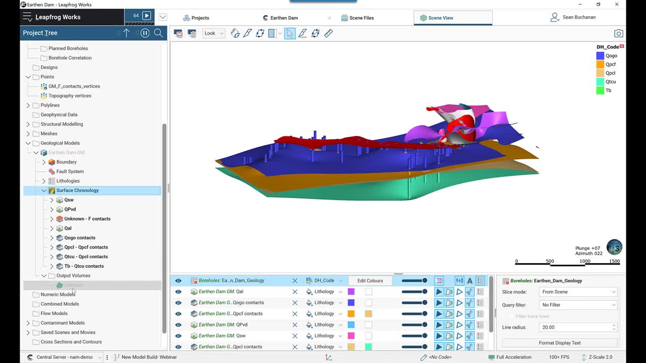
and bring them into the scene.

[00:47:07.840]
And here’s my geologic model.

[00:47:11.110]
So something we’re going to want to do

[00:47:12.270]
is validate this model against our borehole information.

[00:47:15.980]
So I’m just going to click D on my keyboard

[00:47:17.700]
to look directly down,

[00:47:19.060]
maybe change the opacity of these, maybe 50%.

[00:47:22.570]
I’m going to use this slicer tool up in my toolbar

[00:47:25.860]
and cut a slice directly through my model.

[00:47:28.770]
And then I’ll press L stands for look,

[00:47:30.910]
to look directly at that slice.

[00:47:34.190]
From here, I’ll just do a split view

[00:47:36.920]
so I can see where I’m at in my transect,

[00:47:41.120]
and I can now work through my model.

[00:47:42.840]
So I’m just going to press the period on my keyboard,

[00:47:45.140]
which is going to work south.

[00:47:47.560]
Yep, so now I’m stepping south.

[00:47:51.150]
I can change my step width, so right now my step size is 40.

[00:47:54.800]
Maybe I’ll just make it 50,

[00:47:57.160]
and then my slice width, I can also make 50.

[00:48:01.970]
So all that is,

[00:48:05.180]
here’s my slice width,

[00:48:06.410]
that’s actually going to be 25 feet on each side

[00:48:09.720]
or whatever unit you’re working in.

[00:48:12.620]
And then my step size is going to be moving 50 units as well.

[00:48:15.950]
So here I am, just stepping through my model,

[00:48:18.970]
comparing my borehole information

[00:48:20.610]
to my actual output volumes.

[00:48:24.280]
So these seem to be looking pretty good.

[00:48:27.510]
Yeah, we definitely recommend you do some model validation

[00:48:32.160]
after you build your model,

[00:48:33.440]
and this is a fast and easy way to do it.

[00:48:36.480]
So I can just work back again.

[00:48:42.690]
And there’s different slicer modes,

[00:48:44.310]
so I was using fixed slice here, I can remove front,

[00:48:48.950]
so I look around to remove everything in front of my slicer.

[00:48:51.550]
I can do the same for remove back,

[00:48:54.622]
and a few other options here, so pretty fun to explore.

[00:49:00.350]
All right, I’m going to get out of my slicer mode

[00:49:03.520]
and pull in my surface topography

[00:49:05.810]
’cause I do want to create some cross sections

[00:49:09.360]
along our dam access line.

[00:49:13.333]
I’ma go ahead and clean up my project tree.

[00:49:15.390]
So I’m going to right click project trees,

[00:49:17.493]
select collapse rows, just so I’m organized.

[00:49:21.750]
Now I can go into my cross sections and contours folder,

[00:49:25.550]
right click, I can select from quite a few different types

[00:49:29.550]
of cross-section types,

[00:49:31.160]
in this case, I want a new alignment serial section.

[00:49:36.410]
From here, I’ll go ahead and select this existing line,

[00:49:38.930]
which is my dam access line.

[00:49:41.250]
I zoom in on this.

[00:49:42.512]
It’s already started to build some cross section transects.

[00:49:45.840]
So F stands for front, B is for back,

[00:49:48.647]
and these are in a 30 unit (indistinct) spacing.

[00:49:52.300]
So I can change that here.

[00:49:53.682]
It doesn’t really need to be that granular,

[00:49:55.090]
I’ll change it to 500.

[00:49:58.303]
Then I can go in and change the width

[00:50:00.520]
of these cross sections, I’ll say 500,

[00:50:03.810]
height I also put 500.

[00:50:06.380]
Yeah, this will extend a little bit above my topography,

[00:50:08.660]
so I need to adjust that height.

[00:50:10.730]
So I can start moving those down

[00:50:12.680]
to make sure it ends in my basalt unit.

[00:50:15.600]
I think negative 130 will work pretty well.

[00:50:21.880]
So once I’m happy with these,

[00:50:25.410]
I can go ahead and press okay.

[00:50:30.380]
So this is my dam axis too.

[00:50:32.500]
I actually just made one, which I’ll work off of later.

[00:50:38.290]
But to add a new master section layout,

[00:50:41.660]
so I want to add data to this cross section.

[00:50:43.520]
I’m just going to right click, select new master section layout

[00:50:48.650]
and just like the project tree I can right click

[00:50:51.020]
on one of these folders to add data.

[00:50:52.900]
So I’ll just right click on models, select add model,

[00:50:56.930]
and I can add my or the dam to this cross section.

[00:51:05.660]
So that’ll generate pretty rapidly.

[00:51:14.090]
I can also go in and change my X and Y axis.

[00:51:17.680]
So I’ll go ahead and change this to feet.

[00:51:21.760]
Maybe I want a secondary Y axis and I want to use,

[00:51:25.423]
uncheck the real world coordinates.

[00:51:31.110]
Can just move this legend out of the way for now.

[00:51:33.310]
And then to add boreholes, I’ll just right click.

[00:51:36.580]
I’ll add my borings, select the correct table.

[00:51:43.900]
This is going to give me a minimum distance to section point.

[00:51:46.250]
So this is what’s going to project on my cross section.

[00:51:48.970]
Right now it’s giving me 2,000 unit radius to project them.

[00:51:54.260]
It’s kind of a little high for what I want,

[00:51:55.970]
I’m just going to change this to 300

[00:51:58.630]
and make sure these are selected,

[00:51:59.840]
so those will be projected onto my section line.

[00:52:04.520]
From here, maybe I want to show my DH code.

[00:52:07.190]
If I had other attributes that had some downhole data,

[00:52:10.020]
I can also bring those in to show, to be placed on the left

[00:52:13.210]
or the right of the line and go into my points and labels,

[00:52:17.910]
show depth markers, maybe I want my borehole names

[00:52:24.750]
to be at a 45 degree angle, show minimum distance.

[00:52:31.465]
Something I like to do is add in my topo data.

[00:52:34.550]
So I can just right click, add surface,

[00:52:36.240]
bring in my topography.

[00:52:39.400]
Maybe I’ll change this to brown and increase the line width.

[00:52:44.720]
I can also add this to my legend, so I’ll pop over here.

[00:52:48.070]
Any additional lines, points,

[00:52:49.680]
structural data I can also bring in.

[00:52:52.510]
I can easily move these around,

[00:52:55.260]
change some attributes in my legend.

[00:52:59.720]
So really intuitive workflow design here.

[00:53:03.915]
If I’m happy with this mock master layout,

[00:53:06.080]
I can go ahead and press the save button and exit out,

[00:53:10.480]
and then I can apply this master layout

[00:53:12.730]
to all of my other sections.

[00:53:14.660]
So I can just right click on my dam axis,

[00:53:17.000]
and select copy master layout two.

[00:53:20.580]
And I can choose all of these changes, spaced,

[00:53:26.660]
cross sections and press okay.

[00:53:27.817]
And that will reprocess with that master layout.

[00:53:30.880]
So I’ve already done that

[00:53:32.920]
and cleaned up my master layout a bit,

[00:53:38.200]
so we can see what it looks like now.

[00:53:39.740]
I’ve added a image kind of looking down

[00:53:42.310]
on where my cross sections are,

[00:53:43.730]
so I could go in and add an arrow,

[00:53:46.630]
maybe a text box point

[00:53:47.840]
to which transect line we’re looking at,

[00:53:50.700]
or add other attributes to my legend,

[00:53:54.010]
change up my vertical scale, so on and so forth.

[00:53:56.930]
So what’s next here is I can bring all these in

[00:54:02.290]
at the same time, see what this looks like.

[00:54:07.650]
Then I can also export these cross sections

[00:54:10.720]
to be used in other programs like GeoStudio.

[00:54:14.510]
So if I right click here, I can export and export these

[00:54:19.730]
in a few different design files, so DXF, DWG or DGN.

[00:54:25.540]
I can also export these as PNG, SVG, GeoTIFF files,

[00:54:32.680]
to be dumped right into a report.

[00:54:38.738]
Then you can always bring in your geologic model

[00:54:43.240]
and overlay that with your cross sections.

[00:54:54.338]
And that’s all the time we have today.

[00:54:55.630]
Sorry, I really spent a lot of time

[00:54:59.150]
focusing on importing the data,

[00:55:00.950]
then zoom through the rest of this.

[00:55:02.090]
But any questions,

[00:55:03.720]
feel free to ask them now and love to go over them.

[00:55:07.541]
(soft music)