Leapfrog Works 4.0.1 – New look, new integrations and significant performance enhancements

This webinar is the best place to learn how the new functionality can improve efficiency in your workflows, give you more flexibility and help you make decisions faster.

Webinar highlights include:

• Borehole performance improvements
• Calculations on interval tables
• OpenGround cloud integration
• Improved mesh handling
• Central publishing improvements
• And much more!

Overview

Video Transcript

[00:00:01.170]<v Jeff>Welcome to the webinar</v>

[00:00:02.100]for Leapfrog Works version 4.0.1.

[00:00:05.800]My name is Jeff McKeon,

[00:00:07.090]a project geologist with Seequent

[00:00:09.120]based out of Denver, Colorado,

[00:00:11.180]and I will be leading you through the new release.

[00:00:14.980]Here’s an overview of some of the main themes

[00:00:16.910]we will be discussing in this product update webinar.

[00:00:20.190]I will introduce them here,

[00:00:21.570]and describe them in more detail later in the webinar,

[00:00:23.910]along with a demo at the end

[00:00:25.230]to show some of the added features.

[00:00:30.570]Seequent has put a huge amount of effort

[00:00:32.200]into updating the building blocks of Leapfrog.

[00:00:34.360]And this has enabled us to change to a new user interface.

[00:00:41.040]The new user interface is sleek, streamlined,

[00:00:43.810]and brings cohesion across the Seequent range of products.

[00:00:47.630]While it may appear quite different at first glance,

[00:00:50.060]all of the functionality remains in exactly the same place

[00:00:52.730]as it was before.

[00:00:56.500]Secondly, we really wanted to show you the work we put in

[00:00:59.330]to making the Leapfrog user experience better

[00:01:01.990]when using some of the main functionality.

[00:01:04.760]We have made improvements to both borehole data and meshes.

[00:01:10.550]When it comes to borehole data,

[00:01:11.890]we wanted to focus on speed improvements.

[00:01:14.390]So we have made changes to ensure that borehole data

[00:01:16.690]processes much faster.

[00:01:19.680]For meshes, it’s often a struggle

[00:01:21.670]to detect errors in the mesh.

[00:01:24.470]We have improved visibility of these mesh issues

[00:01:26.880]so you can better understand how to fix your meshes

[00:01:29.270]for further use in downstream processes.

[00:01:35.370]So to start,

[00:01:36.203]let’s talk about the borehole data improvements.

[00:01:40.880]We’ve made improvements to processing of tasks in parallel,

[00:01:44.340]so that your borehole data can process and reload

[00:01:46.450]substantially quicker for some projects.

[00:01:49.760]In some instances,

[00:01:50.980]we have reduced the processing time by over 40%.

[00:01:57.330]To make importing your borehole data easier,

[00:02:00.010]you can now import your borehole points

[00:02:01.680]at the same time as your caller, survey, and interval data.

[00:02:08.810]In the previous build,

[00:02:09.960]if you made a mistake importing,

[00:02:11.440]or no longer required one of your data columns,

[00:02:14.230]you were unable to remove it.

[00:02:16.320]The new version of Leapfrog

[00:02:17.420]will now allow you to rename and delete

[00:02:19.360]your imported columns,

[00:02:20.630]which will enable you to keep your data up to date

[00:02:22.830]and relevant.

[00:02:24.710]This option is available for all data tables,

[00:02:26.950]including collars, interval tables, GIS data,

[00:02:29.980]and structural data.

[00:02:33.670]Probably one of the most exciting additions

[00:02:35.770]to the borehole data are calculations.

[00:02:38.860]Use the Calculations tab to write calculations

[00:02:41.350]that will categorize, combine and reclassify your data.

[00:02:47.420]Calculations are also available for calculated points,

[00:02:50.350]such as midpoints, intrusion points and decorative points.

[00:02:58.520]Dealing with meshes with issues

[00:02:59.840]can be extremely frustrating.

[00:03:02.300]It’s often hard to know where the problems are

[00:03:04.380]and how to fix them, which can halt your workflow

[00:03:07.250]and be really time-consuming to diagnose.

[00:03:10.260]This release, we’ve made some changes to make this easier.

[00:03:16.130]Firstly, we’ve improved the way

[00:03:17.710]that we categorize the mesh issues.

[00:03:20.320]Instead of having to look at the properties of the mesh

[00:03:22.900]to see if there’s any CSG errors,

[00:03:25.510]it’s now clear which errors that the mesh contains

[00:03:27.980]from the project tree view.

[00:03:33.050]Secondly, the tick box to view the border edge on a mesh

[00:03:36.080]has now been turned into its own separate object.

[00:03:39.660]This means that you can view

[00:03:40.690]the location of the issue in the scene

[00:03:42.480]independent of the mesh.

[00:03:44.720]The border edges object can also be exported as a line file,

[00:03:47.860]which can be visualized in the source program.

[00:03:52.840]We have also added another categorization

[00:03:55.040]to the way we define non-manifold meshes.

[00:03:58.640]As well as being able to view

[00:03:59.800]the non-manifold edges in the scene as their own object,

[00:04:03.150]we have also enabled some non-manifold meshes

[00:04:05.490]to be used in downstream processes that were once unusable.

[00:04:10.090]While non-manifold meshes

[00:04:11.420]with an odd number of adjoining triangles remain unusable,

[00:04:15.140]if there are an even number of adjoining triangles,

[00:04:18.100]they can now be used in the modeling process.

[00:04:23.970]It is important to us

[00:04:25.030]that you feel like your voice is heard,

[00:04:27.470]which is why we’re happy to announce that for this release,

[00:04:29.920]we’ve addressed some of the most highly requested features.

[00:04:35.630]We’ve listened to your request and added functionality

[00:04:38.290]to ensure that we continue to respond to your feedback.

[00:04:42.670]Visualizing depth in the scene, reordering legend items,

[00:04:46.520]and being able to project a subset of collars

[00:04:48.690]onto the topography are all now possible in Leapfrog Works.

[00:04:54.450]To enhance your understanding of your borehole data,

[00:04:57.140]you can now visualize the downhole depth

[00:04:59.410]of your boreholes in the scene.

[00:05:03.890]To utilize this new feature,

[00:05:05.600]view the borehole trace in the scene.

[00:05:08.430]You can customize the tick size, location, and frequency

[00:05:11.930]to ensure they are visible in the scene

[00:05:13.610]alongside your boreholes.

[00:05:16.160]Clicking on an interval in the scene

[00:05:17.540]will also show the downhole depth in the Properties panel.

[00:05:24.100]Legends are an important method

[00:05:25.710]of communicating your categorical data,

[00:05:28.390]which is why we’ve made changes

[00:05:29.720]to allow reordering of unit codes in your legend.

[00:05:34.940]Open the Edit Colors menu from any category column,

[00:05:37.710]to see the list of legend items.

[00:05:40.170]Use the arrows to change their order

[00:05:41.920]to match the unit chronology.

[00:05:45.420]Changes made to the legend will update subsequent objects,

[00:05:48.880]but you also have the freedom to set a different order.

[00:05:55.620]Making changes to the collar elevation

[00:05:57.590]to match the topography

[00:05:59.410]isn’t something you want to do for all of your collars.

[00:06:02.890]Which is why we’ve implemented the ability

[00:06:05.460]to project a subset of collars onto the topography.

[00:06:11.020]In the new release,

[00:06:12.160]when choosing to set the elevation for your collar,

[00:06:14.750]you can now apply a query filter.

[00:06:17.820]With the addition of a query filter

[00:06:19.470]you can now choose any subset of your collars

[00:06:21.550]to change the elevation of.

[00:06:24.160]Also, you’re not just limited to the topography.

[00:06:27.200]You can choose any surface to project the collars onto.

[00:06:33.350]Creating meshes and surfaces from non-contact points

[00:06:36.330]is now possible with the new guide points.

[00:06:41.402]In this release, we can now create guide points,

[00:06:44.570]use categories on points to classify them

[00:06:46.810]as interior and exterior.

[00:06:49.680]When you make meshes and surfaces,

[00:06:51.260]this information will be used to guide a path

[00:06:53.310]through the interior and exterior,

[00:06:55.670]to guide the creation of your surface.

[00:07:02.520]In this release, we wanted to make

[00:07:04.030]the ties to the Seequent products even stronger

[00:07:06.670]through our interoperability improvements.

[00:07:12.760]Through the OMF,

[00:07:13.640]we can now import 2D and 3D geophysical grids into Leapfrog.

[00:07:18.060]And through Seequent Central,

[00:07:19.340]we can import more than ever from other projects

[00:07:21.740]in the Files tab and the Seequent Central portal.

[00:07:27.200]The Open Mining Format or OMF

[00:07:29.550]is a great way of transferring multiple files

[00:07:31.830]across projects.

[00:07:33.770]With one single OMF file,

[00:07:35.430]you can import all of the necessary objects

[00:07:37.740]to view 2D and 3D geophysical grids in Leapfrog.

[00:07:43.640]Use the Leapfrog Works OMF menu

[00:07:46.240]to import Oasis montaj geophysical grids

[00:07:48.950]from the central data room, or from a file.

[00:07:52.900]Also, imported grids now have improved discrete color maps

[00:07:56.460]to ensure that they will match those in Oasis montaj.

[00:08:03.350]This new release also introduces a new way

[00:08:05.510]of bringing boreholes into your project.

[00:08:11.150]The new Import Boreholes

[00:08:12.430]via OpenGround Cloud connection for works

[00:08:14.970]allows you to connect directly

[00:08:16.460]to the Bentley OpenGround Cloud data.

[00:08:19.890]This way you can be assured

[00:08:21.160]that your data is safe, secure, and up to date.

[00:08:27.230]The ability to collaborate and access data

[00:08:29.650]between files and projects has become far easier

[00:08:32.670]with this new release.

[00:08:34.720]You can use the central data room or existing projects

[00:08:38.070]to collate or import data into your project,

[00:08:41.480]increasing the flexibility

[00:08:42.810]of how you build and manage your projects and data.

[00:08:49.320]The ability to import meshes from other central projects

[00:08:52.310]was a feature of the last release.

[00:08:55.530]We have increased support of objects,

[00:08:57.100]able to be imported from an existing central project

[00:08:59.920]to include structural data, points, and polylines.

[00:09:04.260]Geological models and refined models

[00:09:06.020]can also be imported as static models

[00:09:08.030]from an existing project.

[00:09:12.430]As well as being able to import from other central projects,

[00:09:15.870]you can now import from the central data room of a project

[00:09:19.390]through the Files tab.

[00:09:21.240]Support has been added for many objects,

[00:09:23.160]including points, structural data, and polylines.

[00:09:26.850]You can now upload your borehole data

[00:09:28.450]to the central data room,

[00:09:29.790]and use this as the foundation of your project as well.

[00:09:33.300]Uploading new revisions of your data

[00:09:35.010]will cause the object to appear out of date,

[00:09:36.990]indicated by a small clock icon in your project tree.

[00:09:40.970]This will prompt anyone using the data

[00:09:42.820]to reload to the latest version.

[00:09:46.120]Also, we now have support

[00:09:47.710]so that borehole traces and lineations

[00:09:49.720]can be published to Central.

[00:09:53.000]In the new release we’ve made some changes

[00:09:54.680]to the contaminants extension.

[00:09:57.740]We’ve added additional variogram types,

[00:10:00.770]Gaussian, exponential, cubic, and generalized cauchy.

[00:10:06.390]We have also added a lock sill functionality

[00:10:08.640]to the variogram process,

[00:10:10.590]allowing you to manipulate your range

[00:10:12.350]without unintentionally changing the cell value

[00:10:14.690]for your other axes.

[00:10:16.900]Now that we’ve discussed the new Leapfrog Works features,

[00:10:19.930]I will now demo some of the features for you.

[00:10:24.720]to project a subset of collars onto your topography,

[00:10:28.350]come over to your collar table,

[00:10:30.950]right-click and select Set Elevation.

[00:10:34.680]Here you’ll have the option of applying a query filter.

[00:10:38.380]I have one pre-built titled AB Holes,

[00:10:40.620]so I will select that now.

[00:10:42.720]As well as my typography.

[00:10:46.250]Note that you can also select any other surface types

[00:10:50.150]in your projects to project your collars onto.

[00:10:54.180]Once you’re happy, select OK.

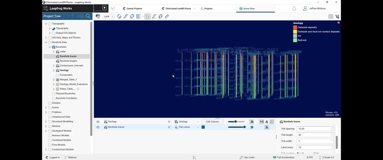
[00:10:59.420]To visualize downhill depth in the scene,

[00:11:02.160]you first want to drag your borehole traces

[00:11:04.190]into your scene view,

[00:11:06.150]come down to the options, and select Show Depth Marks.

[00:11:11.620]If you scroll down,

[00:11:12.453]you can see that you can change these parameters.

[00:11:15.310]So I’m going to change the tick spacing to 10,

[00:11:21.450]the tick length to 30, and label every 10.

[00:11:28.593]And if you look in your CV, you can see that reflected here.

[00:11:32.850]Another feature that was added

[00:11:34.060]is now you can select your borehole.

[00:11:37.370]And see the downhole depth in the scene details.

[00:11:43.270]To reorder your legend,

[00:11:44.650]come over to your lithology table and double-click.

[00:11:48.710]This will populate your legend.

[00:11:51.610]Before it was in alphabetical order,

[00:11:53.360]but now we have the ability to reorder these units.

[00:11:56.700]So just select the unit of interest.

[00:12:01.290]And click on these arrows to toggle it up and down.

[00:12:04.350]When you’re happy, select OK.

[00:12:06.910]And that will be reflected in your legend in the scene.

[00:12:13.090]The points that I have viewable in my scene view

[00:12:15.640]represent my water table.

[00:12:17.620]The pink points are my vadose zone,

[00:12:19.350]the blue points are my saturated zone,

[00:12:21.730]and the gray points are my bedrock.

[00:12:25.050]In previous build, because these are not contact points,

[00:12:27.770]it would be difficult to generate a surface

[00:12:30.270]where the new guide point functionality comes into play.

[00:12:34.470]To create guide points, you simply click on your points,

[00:12:38.730]and select New Guide Points.

[00:12:41.300]This will bring up this box here,

[00:12:42.950]where we can specify if the points are interior or exterior.

[00:12:48.520]I’m going to model a surface

[00:12:49.990]between my vadose zone and my saturated zone.

[00:12:54.380]So I’m going to keep my vadose zone as my interior points.

[00:12:59.160]And move my bedrock and saturated points to my exterior,

[00:13:02.370]and select OK.

[00:13:05.050]That will create this guide points object.

[00:13:09.040]I hide my water level depth,

[00:13:10.620]you can see now

[00:13:11.480]that the red points represent my interior points,

[00:13:14.930]while the blue points represent my exterior points.

[00:13:20.840]To create a surface from these guide points,

[00:13:23.670]I come down to meshes, right-click New Mesh from points.

[00:13:29.540]It will populate this box

[00:13:30.940]where I select the points that I just created,

[00:13:34.550]as well as my model extents.

[00:13:38.070]This is also where you set your surface resolution,

[00:13:40.530]I’m going to pop it down by an order of magnitude.

[00:13:44.200]And select OK.

[00:13:46.387]And that will generate this surface right here,

[00:13:49.160]which we can see transects the boundary

[00:13:52.450]between my vadose zone and my saturated zone.

[00:14:01.630]<v Instructor>To create a new calculation</v>

[00:14:02.930]for one of your borehold tables,

[00:14:04.330]you’re going to come over to the table of interest,

[00:14:07.550]right-click, and select Calculations.

[00:14:11.030]The Calculations tab will then appear.

[00:14:13.670]You’re going to click on this little star on the upper left.

[00:14:17.010]Here you have the option of creating a new variable,

[00:14:19.350]a new numeric calculation, or a new category calculation.

[00:14:23.030]In this instance I’m going to create a category calculation,

[00:14:27.380]and title it Missing.

[00:14:30.710]You want to start off with an if statement.

[00:14:32.720]So type in if and the space button, and this will appear.

[00:14:37.420]I’m going to jump over to my syntax in Functions.

[00:14:41.650]And come down to…

[00:14:43.920]I’m going to build one for

[00:14:45.360]if this specific interval has a value,

[00:14:51.740]it will be assayed otherwise missing.

[00:15:00.740]Once we’re happy with this, there should be no errors,

[00:15:04.850]meaning that this is a valid calculation.

[00:15:09.310]In Leapfrog Works

[00:15:10.720]you do have the option of saving these calculations,

[00:15:13.460]so if you have a complex CPT equation,

[00:15:16.860]you just click on this button here

[00:15:18.810]to export it as an LF calc file.

[00:15:23.530]That way you can import it into any of your other projects

[00:15:26.550]without having to go through the same workflow.

[00:15:31.250]And again, when you’re happy, you click Save

[00:15:33.730]and then that will populate your equation.

[00:15:38.350]And calculations underneath the interval table.

[00:15:44.600]And then you can pull that into your scene view,

[00:15:48.760]and view your calculation in the 3D space.

[00:15:57.460]<v Jeff>To connect to the OpenGround Cloud environment,</v>

[00:16:00.550]start at a new project and come to borehole data.

[00:16:04.170]Right-click and select

[00:16:05.210]Import Boreholes via OpenGround Cloud.

[00:16:09.780]And select your environment.

[00:16:14.610]Here we have multiple projects,

[00:16:16.240]I’m going to select the Quinley test project.

[00:16:24.540]And here it’s just loading that information.

[00:16:35.228]And here we can select the data that we want to pull in.

[00:16:38.530]So in this instance,

[00:16:39.590]I’m going to pull in some interval data,

[00:16:43.070]as well as some CPT data.

[00:16:46.960]Here you select if it’s interval or point data,

[00:16:49.870]for this it’s point, so I’m going to select point.

[00:16:53.750]And click Import.

[00:16:58.150]And then that will bring me to the screen

[00:17:00.790]where I map what the columns are, I’m happy with that.

[00:17:06.190]This is my survey table, my lithology table.

[00:17:11.670]And here is the CPT values,

[00:17:14.570]so I’m going to map these as numeric values, and finish.

[00:17:24.300]And then that will populate

[00:17:25.590]just like any of your other techniques

[00:17:29.090]for bringing in borehole data.

[00:17:33.530]Previously, in other Leapfrog builds,

[00:17:36.270]if a mesh had any issues, you would need to right-click,

[00:17:40.400]select Properties and look for CSG errors.

[00:17:43.720]So we can see here that this is not closed,

[00:17:45.740]and this is not manifold.

[00:17:48.090]Also in previous builds, if this did have any errors,

[00:17:51.350]it couldn’t be used for any downstream processes.

[00:17:54.780]We’ve now fixed that to be able to,

[00:17:57.350]I’m just going to pull this into the scene,

[00:17:58.900]this is an excavation volume.

[00:18:02.160]So now if there’s any errors,

[00:18:02.993]there will be this little black triangle next to it,

[00:18:05.800]if you select this,

[00:18:06.940]you can see that there’s an issue with the border edges,

[00:18:13.410]and there’s an issue with some non-manifold edges.

[00:18:17.030]We’ve now separated these into their own objects,

[00:18:19.390]these are polyline objects,

[00:18:20.740]so if I pull these into the scene,

[00:18:24.360]I’m going to bump up the line radius

[00:18:27.260]so that it’s a little bit more apparent.

[00:18:31.830]We can see the border edges

[00:18:33.020]indicated by this darker green line.

[00:18:36.920]And then those non-manifold edges

[00:18:38.880]shown by these lighter green, more lime green little lines.

[00:18:46.470]And a nice feature is that these can be viewed

[00:18:49.030]independent of the mesh.

[00:18:52.010]These also can be exported by right-clicking,

[00:18:55.370]so that you can bring them back into the origin software

[00:18:57.970]to correct these issues.

[00:19:02.500]To import from Central,

[00:19:03.820]right-click on the object of interest,

[00:19:05.770]I’m going to bring in a geological model.

[00:19:09.150]And go to Import Geological Model from Central.

[00:19:13.555]Here you select the project.

[00:19:17.270]You can also select any branch to pull a project from.

[00:19:21.710]I’m going to pull from this experimental branch

[00:19:24.760]and load this initial model phase two.

[00:19:28.280]You just select import.

[00:19:32.414]That will then be populated

[00:19:33.500]under your geological models folder.

[00:19:36.610]We can see here that this is the model that we pulled in

[00:19:39.530]because it has this little half black, half white circle,

[00:19:44.410]which indicates that it was pulled from Central,

[00:19:47.800]as well as this little shield

[00:19:49.190]that indicates that it is a static model,

[00:19:51.750]so it’s not going to be effected

[00:19:53.070]by the input data in this project.

[00:19:57.850]And here it has all of the same folders,

[00:19:59.970]so we can pull in any of the surfaces,

[00:20:03.180]pull in any of the output volumes for this project as well.

[00:20:10.050]In this specific project,

[00:20:11.400]we pulled the borehole data from the central data room.

[00:20:15.580]You can see that by the little central icon right here.

[00:20:19.890]This also has a little clock icon.

[00:20:22.310]This indicates that the data in the central data room

[00:20:25.450]has been updated,

[00:20:26.620]and that the borehole information in this project

[00:20:29.680]is out of date.

[00:20:32.030]To make this up to date,

[00:20:34.820]right-click and select Reload Latest File Versions.

[00:20:42.900]This will then update all of this borehole information

[00:20:46.870]that is out of date by populating this box.

[00:20:53.430]We’re just going to go through

[00:20:54.920]and check that the mappings are correct.

[00:21:05.420]And here we can see that it’s reprocessing

[00:21:08.650]all of the downstream processes

[00:21:10.430]with this new reloading of the data.

[00:21:17.090]Adjusting the range can be fairly frustrating,

[00:21:19.530]because as you’re adjusting the range,

[00:21:21.240]the sill value will change.

[00:21:23.520]Notice this red number right here,

[00:21:25.330]which is the sill value going up and down

[00:21:27.280]as I’m trying to adjust the range.

[00:21:29.630]And then getting back to that range can be pretty difficult.

[00:21:32.930]That’s why we added the lock cell functionality.

[00:21:36.100]If you click this little lock icon right here,

[00:21:39.280]that will lock your cell

[00:21:40.360]so the only thing changing will be your range.

[00:21:46.640]We’ve also added some new structure types.

[00:21:50.340]You click this dropdown,

[00:21:51.560]previously, we had linear, spherical, and spheroidal.

[00:21:55.070]Now we have Gaussian, exponential, cubic,

[00:21:57.440]and generalized cauchy.