Leapfrog Geothermal 5.0.1 – A new look that brings significant performance enhancements

This webinar is the best place to learn how the new functionality can improve efficiency in your workflows, give you more flexibility and help you make decisions faster.

Webinar highlights include:

• Explore the new interface
• Well data performance improvements
• Calculations on interval tables
• Improved mesh handling
• Estimation management with the new Parameter Report
• Central publishing improvements
• And much more!

Overview

Video Transcript

[00:00:01.840]<v ->Hi everyone and thanks for joining us today,</v>

[00:00:03.820]for this webinar,

[00:00:04.750]about the new release of Leapfrog Geothermal 5.0.1.

[00:00:08.750]My name is Bastien Poux.

[00:00:09.970]I am the technical sales advisor for energy at Seequent.

[00:00:13.540]The objective of this webinar is to introduce you

[00:00:15.520]to the main modeling tools available in Leapfrog Geothermal

[00:00:18.590]and some of the latest improvements for the 5.0.1 release.

[00:00:22.940]For those of you, who already know Leapfrog Geothermal,

[00:00:25.410]you might find an interest in seeing,

[00:00:26.730]the new interface of leapfrog and new functionalities.

[00:00:30.540]Before we get going, just a couple go to meeting logistics.

[00:00:34.590]If you take a look at the go to web dialogue,

[00:00:37.020]you should see a place for questions.

[00:00:39.970]I won’t be answering questions during this webinar.

[00:00:42.350]So please use this questions panel to enter your questions

[00:00:45.270]and I would answer them with a personal email,

[00:00:47.180]after the webinar ends.

[00:00:50.200]These new roads is a big one for Seequent,

[00:00:51.960]in not only looks different,

[00:00:53.300]but it also has some key features

[00:00:54.980]that a lot of customers have been asking for.

[00:00:57.680]This webinar is for the geothermal product only,

[00:00:59.950]but it crosses into the realm of Central,

[00:01:02.430]our cloud-based model management and collaboration solution.

[00:01:06.600]Here is an overview of some of the new features,

[00:01:08.770]we will be discussing in this webinar.

[00:01:11.460]I will introduce them quickly here,

[00:01:13.140]before describing them in more details in the webinar.

[00:01:16.590]Firstly, there is a new user interface.

[00:01:19.570]There’s also some usability improvement,

[00:01:21.950]some well data improvement, a better mesh handling system.

[00:01:26.220]Any improvements in the interoperability.

[00:01:29.430]The new Leapfrog user interface,

[00:01:30.950]is the first thing we want to talk about,

[00:01:32.910]because there is no escaping the fact,

[00:01:34.690]that this looks different than the last release.

[00:01:37.070]Seequent has put a huge amount of effort,

[00:01:39.370]into updating the building blocks of Leapfrog

[00:01:41.970]and this has enabled us to change to a new user interface.

[00:01:46.025]The new user interface of Leapfrog is slick streamlined

[00:01:48.930]and brings cohesion across the Seequent range of products.

[00:01:52.420]Even though it may appear quite different at first glance,

[00:01:54.970]with new colors and icons, the layout, the functionalities

[00:01:58.450]and the menus remained the same they were before.

[00:02:01.600]Secondly, we really wanted to show you,

[00:02:03.770]the work we have put,

[00:02:04.680]into making your only Leapfrog experience better

[00:02:07.040]when using some of the main functionalities.

[00:02:09.640]We have made improvement to both well data and meshes.

[00:02:13.530]Let’s talk about the well data improvements.

[00:02:16.540]We’ve made improvements,

[00:02:17.540]to the processing of tasks in parallel,

[00:02:20.070]so that your well data can process

[00:02:21.830]and reload significantly quicker for some projects.

[00:02:25.040]In some instances,

[00:02:26.150]we have reduced the processing time by over 40%.

[00:02:29.760]You can now import down hold points

[00:02:31.360]at the same time as your location, survey and intervals.

[00:02:34.830]If you made a mistake when importing

[00:02:36.680]or no longer require one of your data columns,

[00:02:39.240]you can now rename it or delete it.

[00:02:41.930]Finally, use the calculation tab to categorize, combine

[00:02:45.930]and reclassify your data.

[00:02:48.220]Dealing with meshes that have issues can be difficult.

[00:02:50.690]It is often now to know where the problem is to fix it.

[00:02:53.920]This really is, we have made some changes

[00:02:55.750]to make it easier for you.

[00:02:57.260]Firstly, we have improved the way,

[00:02:58.840]that categorize the mesh issues.

[00:03:01.140]It is now clearer with errors,

[00:03:02.780]that the mesh contains from the tree view,

[00:03:04.820]instead of having to look at the properties of the mesh.

[00:03:07.890]Secondly, the tick box to view the border edge on the mesh

[00:03:11.330]has not been turned into its own separate object.

[00:03:14.400]We have added another categorization

[00:03:16.310]to the way we define non Manny formations.

[00:03:18.890]We have a soul enables, so now many fall meshes to be used,

[00:03:22.410]whereas they were not usable before.

[00:03:24.960]We have listened to your requests and added functionalities,

[00:03:27.900]to ensure that we continue to respond to your feedback.

[00:03:31.280]Visualizing depth in the scene, reordering legion item

[00:03:34.700]and being able to project a subset of the locations

[00:03:37.400]onto the typography, are all now possible,

[00:03:39.850]in Leapfrog Geothermal 5.0.1.

[00:03:42.909]I will show you these functionalities,

[00:03:44.520]in the software in a moment.

[00:03:46.550]You can now view the well traces in the scene

[00:03:48.670]and choose to show the depth markers.

[00:03:51.280]You can also customize how often these ticks are labeled

[00:03:54.450]and how big thy are, to ensure that you can still see them,

[00:03:57.090]alongside your weld data.

[00:03:59.240]Also to enhance your understanding of your world data,

[00:04:02.390]you can now visualize the downhole depth,

[00:04:04.540]of your well data in the scene.

[00:04:06.630]Legends they are the most important method,

[00:04:09.430]of communicating your category data.

[00:04:12.030]We have made changes that you can now reorder

[00:04:14.170]your unit codes in the legend.

[00:04:16.360]Displaying well data on the cross section,

[00:04:18.530]will adopt the same legend order as your base color.

[00:04:21.670]Making changes to the location elevation

[00:04:23.690]to match the typography, is not always something

[00:04:25.990]you want to do for all your wells.

[00:04:27.980]In this new radius,

[00:04:29.200]when choosing to set the elevation for your location,

[00:04:31.880]you can now apply your query filter

[00:04:33.690]for any subset of your location

[00:04:35.780]to change the elevation off.

[00:04:37.650]You’re not just limited to the topography,

[00:04:39.710]you can actually choose any surface

[00:04:41.300]to project the location zone.

[00:04:44.020]Let’s now look at the improvements in central

[00:04:46.610]where the ability to collaborate and access the data

[00:04:49.080]between files and projects

[00:04:50.650]has become far easier with the new release.

[00:04:53.550]You can use the central data room or existing projects

[00:04:56.760]to collate or import data into your project,

[00:04:59.490]increasing the flexibility on how you build

[00:05:01.730]and manage your projects and data.

[00:05:04.010]The ability to import meshes from other central projects

[00:05:06.850]into your own, was a feature of the last release.

[00:05:10.010]We have increased support of objects,

[00:05:11.670]able to be imported from an existing central projects

[00:05:14.800]to include structural data, points and poly lines

[00:05:18.420]and geological model and refined models.

[00:05:21.550]As well as being able to import from other central projects,

[00:05:24.790]you can now import from the data room

[00:05:26.390]of a projects for the files tab.

[00:05:28.780]Support has been added for many objects, including points,

[00:05:31.820]structural data and poly lines.

[00:05:34.190]You can now upload your well data into the central room

[00:05:36.930]and use this as the foundation of your project.

[00:05:39.900]Uploading new revisions of your data,

[00:05:41.460]will cause the object to appear out of date.

[00:05:44.190]Anyone using your data will then know,

[00:05:46.290]to reload to use latest version.

[00:05:48.880]That is it for the description

[00:05:50.020]of the new functionalities Leapfrog Geothermal.

[00:05:52.780]I will now jump into the program

[00:05:54.290]to give you a general overview,

[00:05:55.680]of what can be accomplished in leapfrog

[00:05:58.140]and how some of these new functionalities work.

[00:06:03.330]All right, we are now into Leapfrog Geothermal.

[00:06:06.580]This is using the last version 5.0.1,

[00:06:09.960]with its new interface.

[00:06:12.300]Some of you that already use Leapfrog Geothermal,

[00:06:15.160]might see the difference in also the icons on the left

[00:06:19.430]and the folders.

[00:06:21.140]So as a general overview of the interface,

[00:06:25.090]you have on the top left here,

[00:06:26.690]the Leapfrog Geothermal menu,

[00:06:28.800]on the left here is the product tree.

[00:06:31.000]So that’s where you would import all your object,

[00:06:33.920]that’s where you will create your geological model

[00:06:36.650]and create different export formats,

[00:06:39.430]like cross sections or movies.

[00:06:42.430]In the middle here, you have the 3D scene,

[00:06:44.370]right now we can see this saturity meshed,

[00:06:47.240]draped on the topography.

[00:06:49.750]Right above it, is a simple toolbar to slice your model,

[00:06:54.050]to divide it in different windows.

[00:06:57.610]Below the 3D scene, you have the shape list.

[00:07:00.170]So all the objects that are in the 3D scene,

[00:07:02.810]will be listed here.

[00:07:05.010]You can change their coral skin, their transparency

[00:07:08.590]and if you select them,

[00:07:10.270]then you have a property panel here on the right

[00:07:13.030]that allows you to change the slice mode, to filter,

[00:07:17.660]to change the size of the symbols, for example.

[00:07:23.620]So when you want to bring a new object that you imported

[00:07:26.670]or created in Leapfrog, it’s pretty easy.

[00:07:29.360]For example, let’s take some well data

[00:07:30.980]and we’re going to take the geology.

[00:07:32.270]So you just grab it and you drag it into the scene

[00:07:35.810]and they will be displayed.

[00:07:39.670]So to make it easier for this webinar,

[00:07:42.380]I have prepared in advance,

[00:07:45.030]a series of scenes already made,

[00:07:48.660]with a selection of objects in them.

[00:07:51.290]So we’re going to start with the basics.

[00:07:54.140]So this is for the scene of the topographic.

[00:07:58.090]So you see here in the background my digital elevation model

[00:08:00.960]that was imported and every data from the surface

[00:08:04.530]that I would important into Leapfrog would be draped on it.

[00:08:09.090]So for example, you can have a geological map,

[00:08:14.070]or it could be a satellite image.

[00:08:19.600]You can combine images with, for example, GIS objects.

[00:08:25.140]So, we’re going to look at the rivers, the road

[00:08:32.070]and we still have this saturity image in the background

[00:08:35.850]and you can add more GIS objects, for example,

[00:08:38.200]alterations zones or some lease boundaries.

[00:08:43.775]These are types of data that you will import for example,

[00:08:47.210]are geophysical data.

[00:08:50.160]So there are different formats,

[00:08:51.840]that you can import in Leapfrog Geothermal,

[00:08:54.440]the simple ones or for example,

[00:08:56.210]those 2D grids from OS motor, this is the gravity.

[00:09:01.570]Other types of data that you will need to important,

[00:09:03.930]that are very relevant to geothermal,

[00:09:06.220]are the magnetotelluric 3D grids.

[00:09:09.010]So here is an example of one.

[00:09:11.590]So this is directly from the Investran software,

[00:09:14.690]but you will be able to apply value filter on it.

[00:09:18.140]So this is up to 10 on permitter.

[00:09:21.760]So we can see the low resistivity areas

[00:09:26.410]or you can also apply index filter in the free directions,

[00:09:30.480]which will slice your model.

[00:09:34.020]And then you can move inside the model

[00:09:36.670]to visualize different areas.

[00:09:40.870]From this 3D grid you can also extract ISO surfaces.

[00:09:45.989]So that’s a tool in Leapfrog,

[00:09:48.050]using the inverse distance weighted interpolation,

[00:09:52.290]where you would be able to select a series of ISO surface

[00:09:59.210]from the value you wish to see.

[00:10:01.090]And this would create ISO surfaces

[00:10:02.600]that can be reused later in the geological model

[00:10:06.000]or conceptual model.

[00:10:08.636]Also formats that you can import involve, for example,

[00:10:12.710]some density model resulting from VOXI inversions.

[00:10:17.870]So we see it here as a grid,

[00:10:23.780]that was imported in Leapfrog

[00:10:27.340]and the same way as we did for the magnetotelluric.

[00:10:30.690]You can also create from it different ISO surfaces.

[00:10:39.390]Removed VOXI.

[00:10:45.530]Lastly and those are type of geophysical data,

[00:10:48.300]that you can import in Leapfrog are,

[00:10:52.330]the microseismicity data.

[00:10:55.560]So here what we see is a bunch of earthquakes,

[00:10:59.770]that took place over almost 10 years in this project area

[00:11:05.300]and they are sized by magnitude.

[00:11:08.020]So the rate spheres represent

[00:11:10.610]the highest magnitude earthquakes in this region.

[00:11:14.240]You can filter them.

[00:11:15.970]For example, we only want to see the earthquake,

[00:11:18.860]that have a magnitude of both free.

[00:11:25.300]So there’s only a few,

[00:11:26.590]or you can filter them by the time also

[00:11:28.630]because you imported those earthquake data

[00:11:31.200]with the time they happened down to the seconds, possibly.

[00:11:35.410]And you can filter with this tool,

[00:11:38.000]you have a little calendar, so you can change the date.

[00:11:41.400]So we can go down to only a few hours

[00:11:44.910]and then you can visualize the time series of the events,

[00:11:51.830]or you can limit them to a small time, for example,

[00:11:54.580]if you were injecting or if you were dreading,

[00:11:56.800]you can see a cluster here of earthquakes in this region.

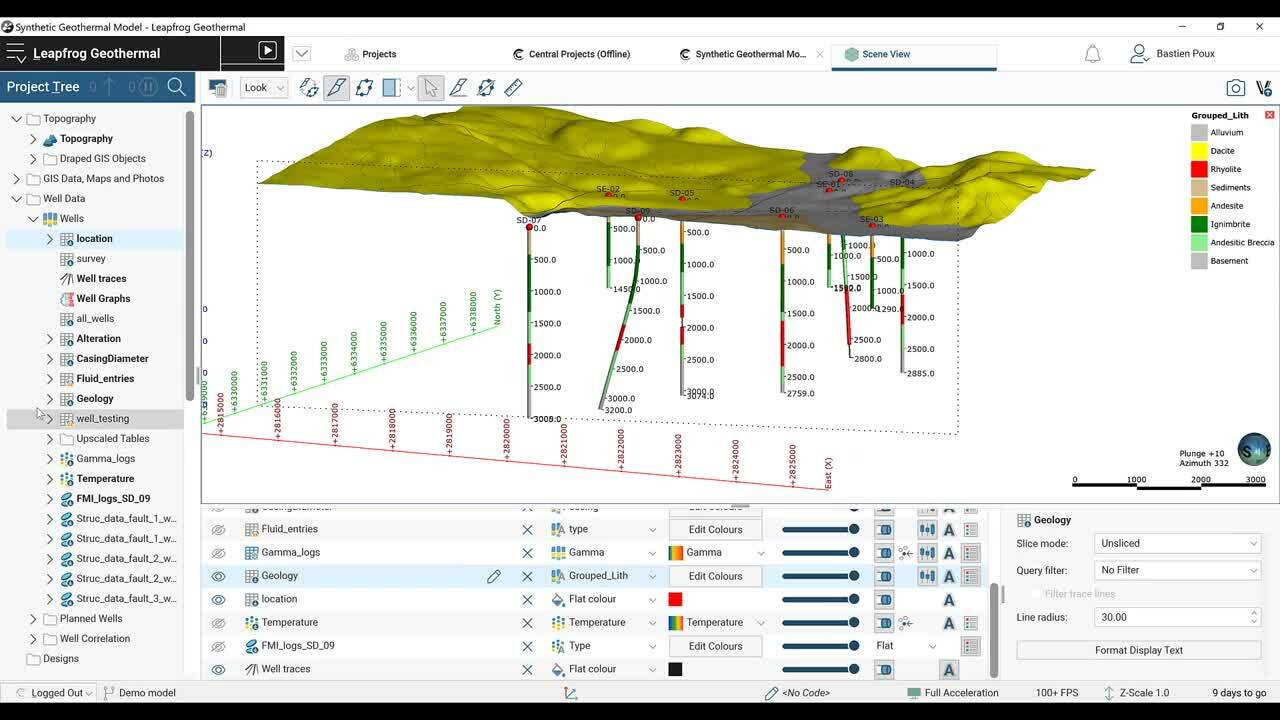
[00:12:03.300]Some of the most important data that you can import,

[00:12:05.890]will be the well data.

[00:12:09.300]So here, this is one of the new functionality of Leapfrog,

[00:12:12.180]where you can see the depth along the well in 3D

[00:12:16.540]and anywhere you click on the well,

[00:12:18.920]you see this little blue cone marker here,

[00:12:21.450]it gives me the downhole depth.

[00:12:22.960]So if I want to select any part of the well,

[00:12:27.000]I can see right here the downhole depth

[00:12:28.927]and this is a major improvement for your workflows,

[00:12:31.170]it will definitely makes things much easier.

[00:12:37.087]Another thing to know now is,

[00:12:39.150]this legend here on the right.

[00:12:41.230]We’re not able before to do that,

[00:12:42.700]but now you can actually change the orders of the unit

[00:12:47.320]and it will adapt.

[00:12:48.820]So this will be much easier for you

[00:12:50.740]to create figures from Leapfrog.

[00:12:54.740]Also, you were able before to protect directly

[00:13:00.156]your locations, your surface location of the wells

[00:13:03.560]on the topography.

[00:13:05.210]Well, now what you can do is actually you can project them,

[00:13:09.330]on any surface, but also you can use query filter

[00:13:13.170]to select only certain of your wells

[00:13:15.720]and then you can select on which surface,

[00:13:17.490]you want to protect them.

[00:13:21.230]So where would these wells be used for?

[00:13:25.220]First, you can use, for example,

[00:13:27.670]if you have the geology like this,

[00:13:29.710]you can create geological model and different surfaces,

[00:13:33.380]like I will show you after.

[00:13:36.047]But first, I want to show you the different types of well data

[00:13:38.453]they can visualize.

[00:13:39.880]So here is the geology.

[00:13:42.330]We can also look for example, at the casing of your wells,

[00:13:49.860]you can add some other information like the fluid entries

[00:13:54.310]to see where are your most predictive zones.

[00:13:59.000]Other types of data you can look at,

[00:14:01.840]we, for example, temperature measurements,

[00:14:05.430]presented here as parents.

[00:14:09.040]You could have some geophysical logs,

[00:14:11.340]here are the Gamma ray logs.

[00:14:15.820]And you can also visualize them as graphs

[00:14:18.850]on the side of the well,

[00:14:19.690]so this allows you to look at a bunch of data

[00:14:22.450]at the same time, super, super posed a lot of data

[00:14:26.670]to create some graphics.

[00:14:30.690]So if I wanted to use,

[00:14:36.480]these wells to create surfaces for my geological model,

[00:14:39.903]this is pretty simple.

[00:14:41.990]So there’s a powerful implicit modeling tool in Leapfrog,

[00:14:47.860]called the radial basis function.

[00:14:49.780]So when you create a new geological model,

[00:14:54.230]so here we’re going to create a geological model

[00:14:56.310]from my lithology, change the resolution

[00:15:02.760]and then we’re going to select a smaller area,

[00:15:05.180]so I would just select the area of my wells.

[00:15:10.978]To geology.

[00:15:12.430]All right, so we have the smaller area.

[00:15:16.530]Can change the size of the box

[00:15:18.170]in which you’re going to build your model

[00:15:19.700]and this can even be done later once your model is complete.

[00:15:25.320]And this is going to create a new object here, GM,

[00:15:28.930]where it defines the boundary of my geological model.

[00:15:33.210]So this is the box,

[00:15:34.100]in which I will create my geological model.

[00:15:40.230]And then I can define the fall system,

[00:15:43.100]the lithologies were selected based on my wells.

[00:15:48.470]And I can create different surfaces,

[00:15:50.620]so deposits, erosion, veins or vein system,

[00:15:54.950]you can do stratigraphy.

[00:15:57.310]So this will depend on your geology of your project.

[00:16:02.400]So here we’re going to create,

[00:16:04.120]first we’re going to do a simple fault.

[00:16:06.660]So we have the geological map

[00:16:08.730]and we’re going to create that fault that’s here on surface.

[00:16:11.970]This is fault number free.

[00:16:16.696](indistinct)

[00:16:18.960]All right, so fault number three in red.

[00:16:21.090]So we’re going to use this GIS line on surface

[00:16:23.690]to create a new fault.

[00:16:26.070]So I’m going to create a new fault from a GIS vector data.

[00:16:30.960]And here I will look for my fault number free.

[00:16:36.640]So now the software will calculate a surface

[00:16:38.460]using this line.

[00:16:40.010]So right now it only has the information on surface,

[00:16:42.560]so it’s almost vertical, but I can easily add some data,

[00:16:47.310]to create some angles to my fault.

[00:16:51.060]So I will eat my fault with some structural data.

[00:16:53.510]Those could be data that you import it from your fieldwork,

[00:16:56.560]but in that case, I’m just going to draw one.

[00:16:59.490]So I’m going to go somewhere here in the valley.

[00:17:03.150]And so what I’ve done is,

[00:17:08.830]created this little structural disc

[00:17:12.510]and then I can change this dip,

[00:17:13.620]so we’re going to do something like 80°, all right.

[00:17:19.380]And when I save,

[00:17:21.650]the software will actually recalculate the fault

[00:17:24.370]and make it deep.

[00:17:26.400]All right.

[00:17:27.630]So this is how you create your fault

[00:17:29.280]and then you can create all your fault

[00:17:31.130]and say how each of them interact with the other,

[00:17:34.730]which one’s top on which one.

[00:17:37.540]Just going to stop to this one for this example

[00:17:40.480]and I’m going to create a survey.

[00:17:41.860]So I’m going to create one of the lithology,

[00:17:44.440]so between the in and bright and the end deposit pressure.

[00:17:48.360]So I would simply create here a deposit from my lithologies

[00:17:54.060]and I will select my en embryat,

[00:17:55.390]and the contact pillows with my andestic breccia.

[00:18:01.527]Leapfrog will create this surface

[00:18:04.410]that goes through the wells.

[00:18:06.390]So this is the first interpretation,

[00:18:08.330]but I can totally edit this manually.

[00:18:11.620]So I can draw, I can edit with a polyline

[00:18:17.140]and the way to do this will be,

[00:18:19.090]I will look at my model from above,

[00:18:22.430]make a slice where I want to draw,

[00:18:24.750]so for example, here, this surface,

[00:18:27.960]we’re going to draw simply our polyline here,

[00:18:32.949]see it’s going horizontal and save

[00:18:36.180]I’m going to see my surface is going to adapt to automatically,

[00:18:39.110]to match both the well data

[00:18:41.730]and this polyline that I just drew.

[00:18:48.320]Right now, it doesn’t show any offset,

[00:18:50.620]but I can simply go into my fault system

[00:18:54.380]and activate my fault and this will recalculate,

[00:18:58.920]a surface on each side of the fault actually.

[00:19:02.790]So here I go.

[00:19:05.550]And if I hide my fault,

[00:19:07.970]you see that it has calculated an offset,

[00:19:09.600]based on the data on both sides.

[00:19:11.610]You don’t have to actually, you can have a lithology that,

[00:19:16.030]doesn’t take in account the fault.

[00:19:18.110]So for example, you can say that one of your lithology

[00:19:21.580]is not affected by this fault because it’s more recent

[00:19:24.780]and you can create surfaces like this,

[00:19:26.560]that will not take the fault in account

[00:19:30.250]and will just consider all the data available.

[00:19:33.000]So this one is an intrusion, for example.

[00:19:37.850]So once you create all your surface,

[00:19:39.610]you activate all your fault.

[00:19:42.010]You end up with a nice looking geological model,

[00:19:46.170]like this one, where you see yellow different fault

[00:19:49.020]and the fault intersections, the wells,

[00:19:51.400]different intrusions, the fault offsets,

[00:19:54.400]some faults have no offset in some lithologies.

[00:20:02.250]So this is, how you can create,

[00:20:03.560]some very complex geological model

[00:20:05.090]with much more wells than this,

[00:20:06.793]this is just as an example here.

[00:20:10.970]Now you can create also what we call numerical models.

[00:20:13.730]So this is when you have any type of numerical data

[00:20:16.620]like temperature, pressure, or geochemistry for example,

[00:20:20.730]you will create some ISO surfaces, arrange your data.

[00:20:25.200]So for this example, I will take care of the temperature.

[00:20:28.640]So those are my temperature logs in my wells

[00:20:31.230]and I will create a numeric model.

[00:20:37.590]So we’re going to be working on the temperature data

[00:20:43.340]and we are going to select temperature for the box,

[00:20:47.950]we’re just going to create a model in this small area.

[00:20:54.050]We’re not over the resolution.

[00:20:58.290]And okay.

[00:21:00.350]By default it’s going to create free ISO surfaces,

[00:21:05.230]but we are going to manually change

[00:21:07.780]which value we want to see.

[00:21:09.210]So in the output, I will select 100, 150, 300

[00:21:17.790]and then I will add 250 and 300.

[00:21:23.270]So I will create five different ISO surfaces.

[00:21:25.560]So it’s going to reprocess and I have my ISO surfaces here.

[00:21:34.410]I can look at them and see.

[00:21:37.740]The same way this can be edited, this is the first base.

[00:21:41.650]So you have different way to edit your numeric models.

[00:21:44.650]You can either go into the properties of the interpolant

[00:21:48.360]and change the type of interpolant, change the drift,

[00:21:52.010]the range, you can also apply your trend,

[00:21:57.042]or you can manually decide,

[00:21:58.690]to change the behavior of those surfaces.

[00:22:02.640]So for example, the same way as the geological model

[00:22:06.030]we did for our surface, we’re going to do for temperature.

[00:22:09.150]So the yellow here correspond to temperature of 200°.

[00:22:14.920]So I’m going to be trolling at 200°.

[00:22:24.890]So we see here an area, for example,

[00:22:27.980]here we’re going to be drawing

[00:22:35.460]and we’re going to give to be area, hectares.

[00:22:40.120]Then I save and it’s going to recalculate,

[00:22:41.790]not only my 200° ISO surface,

[00:22:44.010]but it’s going to adapt the ISO surfaces

[00:22:47.390]based on this temperature data.

[00:22:50.090]So you can manually edit,

[00:22:52.070]with a lot of flexibility or temperature models.

[00:22:58.760]So this is the different types of model you can create,

[00:23:00.940]but then using the different data and models you created,

[00:23:05.300]you can actually see how they connect to each other.

[00:23:08.430]So for example, what we did, is we evaluated

[00:23:12.880]our temperature model directly on the fault.

[00:23:16.510]So what you see,

[00:23:17.620]is the temperature distribution on the fault.

[00:23:20.460]So this is very useful when you want to draw a new well

[00:23:23.600]to target the hottest area, where there is a fault.

[00:23:27.820]You can do the same thing on a lithology.

[00:23:33.610]So for example,

[00:23:34.443]this is the temperature distribution on my basement.

[00:23:40.380]Leapfrog is also very useful to create conceptual model

[00:23:43.530]because all those data you integrated in Leapfrog,

[00:23:46.260]you can actually visualize them in the same scene.

[00:23:50.590]So to create is usually used a lot in geothermal

[00:23:55.380]as a conceptual model.

[00:23:56.570]So we see here, the low resistivity clay cap,

[00:23:59.900]we have the main temperature ISO surfaces,

[00:24:03.960]to show us this areas of higher heat flow.

[00:24:08.200]And we look at the temperature distribution on the wells.

[00:24:11.110]We have the fluid entries,

[00:24:12.780]all that allows you to better understand your resource.

[00:24:15.800]So we could imagine some flow coming for that fault

[00:24:18.650]and more permeability at the 40 intersection here.

[00:24:22.310]So if you were to draw new Wells, for example,

[00:24:25.010]this would be very useful to target your new well,

[00:24:28.120]below the clay cap, hot and permeable area.

[00:24:33.600]But this is what we are going to do now.

[00:24:38.300]So with this scene, we selected two faults,

[00:24:41.860]that we think are the most promising for the new well

[00:24:45.390]and we are going to draw a new well here.

[00:24:49.520]So there is a well planning tool in leapfrog,

[00:24:53.690]directional well planning tool.

[00:24:57.930]And when you build a well,

[00:25:01.510]you can create different section for your well.

[00:25:04.190]And for each of the sections,

[00:25:05.410]you can define the type of section.

[00:25:08.030]So you’d have building an angle,

[00:25:10.250]or you’re going to build an angled

[00:25:11.940]and then hold the same as emit an inclination

[00:25:15.440]for a certain distance or the opposite.

[00:25:19.150]So in that case, in those free caves,

[00:25:20.820]you define the target and then you adapt your well design.

[00:25:24.150]In the case, you want to design your well

[00:25:26.110]and see where it goes,

[00:25:27.410]you can also build to land,

[00:25:28.970]which means that you’re going to define the land for section

[00:25:31.590]and then to build up rate and the estimate,

[00:25:35.060]or you going to define the inclination you want to reach

[00:25:38.830]and the build up rate and you going to see where it brings you.

[00:25:45.210]So we’re going to do pretty simple well here.

[00:25:48.810]What you start by doing is you going to say,

[00:25:51.670]where your well is on surface,

[00:25:53.320]so we’re going to put it here.

[00:25:56.390]So my weight is starting here

[00:25:58.607]and it is starting right now with a hundred meters vertical.

[00:26:02.680]That is usually in geothermal.

[00:26:04.740]We’re going to make it a bit longer.

[00:26:06.950]So now we have 500 meters.

[00:26:14.115]We going to make it a bit larger, so that we see better, right.

[00:26:19.580]So for the next section, what we’re going to do is easily,

[00:26:22.950]just build an angle and hold to a certain target.

[00:26:25.680]So here I can just select in my fault is in anywhere

[00:26:30.410]and that’s where my well is going to go.

[00:26:34.960]First to hold, sorry, 500 meters.

[00:26:39.370]And then I create a new section

[00:26:41.300]and this new section is going to be the build and hold.

[00:26:44.550]In here I select where I want to go.

[00:26:47.340]And here I can now change the door I crate.

[00:26:52.840]And if I want after that, I can add another section,

[00:26:56.940]that’s going to be hold to make sure I go through my fault

[00:27:00.100]to managing certainty and I will add 300 meters.

[00:27:06.920]So now I’m passing through the fault, okay.

[00:27:09.740]At any time I can change the target of my section

[00:27:14.040]and the design is going to adapt.

[00:27:20.249]In the case I don’t want to select the target.

[00:27:23.830]I can also just build to a certain inclusion,

[00:27:29.150]so after my 500 meters vertical,

[00:27:32.280]I’m going to build at a rate of 2° per 30 meters,

[00:27:36.250]to reach a target inclination of 50

[00:27:41.930]and target azimuth will be something,

[00:27:44.930]yeah, 260 is pretty much a direction of the fault.

[00:27:49.420]So it’s creating my section

[00:27:52.040]and then after that, I can add a new section into hold.

[00:27:57.170]If I do for a long distance,

[00:27:58.858]I’m likely going to go for my fault.

[00:28:03.220]This can be changed at any time,

[00:28:04.590]if I want to change the buildup rate,

[00:28:06.580]you can see the well will adapt

[00:28:09.660]and I can also change the azimuth.

[00:28:13.530]Am I, whether you going to turn.

[00:28:17.270]So we’re going to make it go for the fault,

[00:28:19.910]260 will go for the fault.

[00:28:23.810]So on plan well number one,

[00:28:26.720]what I have done is I’ve erected my geological model.

[00:28:31.130]So now you can see on it,

[00:28:32.430]the expected lithologies we’re going to encounter

[00:28:34.560]when we drill the well.

[00:28:38.170]And I can also look for example,

[00:28:39.660]the temperature distribution,

[00:28:42.080]that’s going to be lower.

[00:28:43.020]So this way I can find what would be the best well location

[00:28:47.010]to rect maximum temperature.

[00:28:52.250]And these wells can also be exported as a drilling plan.

[00:28:55.800]So with the typical values and data that are required

[00:29:00.290]for drilling engineers to plan the drilling.

[00:29:07.470]you can also easily create cross sections in Leapfrog.

[00:29:12.010]So here is an example, this one is in the 3D scene.

[00:29:17.143]How is the legend?

[00:29:20.660]But you can also create, export some PDFs.

[00:29:27.570]So you created cross section in 2D

[00:29:29.800]and here you see the wells, the temperature,

[00:29:32.400]ISO surface, the lithology

[00:29:34.380]and you will be able to export this as a PDF,

[00:29:39.140]but also you can do a PNG or geo GIF,

[00:29:41.430]so that it will be already geo referenced.

[00:29:45.230]Those sections don’t have to be planner.

[00:29:49.490]You can actually also create some fence section,

[00:29:57.800]with have different sections in them.

[00:30:02.214]And also very useful tool in Leapfrog Geothermal,

[00:30:05.030]is the possibility to export into different formats

[00:30:08.660]for flow simulations.

[00:30:10.520]So currently we have mold flow, fee flow, TOUGH2,

[00:30:13.570]So you can convert in those three formats,

[00:30:15.150]but we can also import a Tetrad models.

[00:30:18.750]So when you create TOUGH2.

[00:30:25.117]You’ll take your geological model and you will convert it,

[00:30:28.820]you will define these grids,

[00:30:29.810]so it can be smaller blocks in the middle,

[00:30:32.330]in the center of your projects of your projective area

[00:30:35.440]and larger blocks on the outside.

[00:30:37.680]So here we see blocks based on the lithologies,

[00:30:41.240]but you can also add defaults

[00:30:44.460]so that we can define different parameters for the faults,

[00:30:47.480]but also see other four of them fourth intersections.

[00:30:52.440]So when you create your TOUGH2 model,

[00:30:56.280]so you have the possibility to integrate here,

[00:30:59.410]all the parameters of your different lithologies,

[00:31:03.330]so in design decide and you will define the density,

[00:31:05.940]the permeability in the three directions, specific heat,

[00:31:09.750]the pressure, but you can also do the same for the fault

[00:31:12.696]and the fault intersection,

[00:31:13.770]because they have different permeability

[00:31:15.910]than the lithologies.

[00:31:20.320]You can also input all the parameters

[00:31:22.170]for your flow simulation.

[00:31:23.300]You define the different type of TOUGH2 engine

[00:31:26.090]and then you will have here all the parameters

[00:31:28.750]cut it as it is in TOUGH.

[00:31:31.725]There you can integrate and the boundary quotations,

[00:31:34.710]if you have any wells with predictive areas,

[00:31:38.730]you can enter them as generators.

[00:31:40.720]And this can be exported as a TOUGH2 input,

[00:31:44.570]so that you can go ahead with,

[00:31:46.570]your history matching and forecasting.

[00:31:50.280]This is a regular grid of TOUGH2 above.

[00:31:52.820]You can also create some irregular Voronoi grinding,

[00:31:58.950]depending on the types of model that you prefer.

[00:32:08.630]And once you have a new simulation,

[00:32:11.010]you can reimport the output results here directly.

[00:32:16.420]So I don’t have for this example,

[00:32:17.860]but I got another project,

[00:32:20.780]where we have the result of the simulation.

[00:32:23.710]So this is similarly geological model on the grid

[00:32:27.130]with only two faults.

[00:32:29.350]And when you reimport the output,

[00:32:32.730]you will be able to select the different parameters

[00:32:35.860]that have been simulated.

[00:32:37.610]So for example, if you look at the pressure,

[00:32:40.670]we’re going to go where our wells are.

[00:32:44.290]So I’m going to flat slice through the wells.

[00:32:53.400]And when we move through time,

[00:32:55.790]we’re going to see that there is a pressure drop

[00:32:58.650]in this reservoir, during the time simulated.

[00:33:03.320]The same way, besides the pressure,

[00:33:06.870]another good one to look at, will be the gas saturation.

[00:33:10.320]So the steam and liquid water.

[00:33:13.160]So if I remove the liquid water, all I see is just a steam

[00:33:18.400]and I can see that in relation to the drop in pressure,

[00:33:22.610]during the time of simulation,

[00:33:24.870]there will be an increase in the steam,

[00:33:29.920]in the top of the reservoir.

[00:33:33.090]For the second part of this webinar,

[00:33:34.600]I will give you a quick overview of Seequent central

[00:33:37.110]and the new improvement with these new release.

[00:33:40.820]First, in the online web portal,

[00:33:43.480]this is where you can access your projects

[00:33:45.240]and manage your users.

[00:33:46.990]If I go back into my geothermal model,

[00:33:50.070]I will access a history of all the past publications,

[00:33:53.280]with their date and the author.

[00:33:55.690]I can also manage the users for this particular project

[00:33:58.750]and change their level of access.

[00:34:02.500]I can also look and share some files,

[00:34:05.540]such as geological map, PDF reports,

[00:34:09.610]or any other types of formats,

[00:34:11.340]it doesn’t have to be Leapfrog specific.

[00:34:14.010]And it also does version control on these files

[00:34:16.890]that you upload.

[00:34:18.620]Here we can see there are different version,

[00:34:20.080]of this geological map.

[00:34:22.680]Now let’s have a look at the browser.

[00:34:26.000]The central browser allows every team member,

[00:34:28.040]to access the models that have been published

[00:34:30.180]and visualize them in a 3D environment.

[00:34:32.580]We don’t need the Leapfrog Geothermal license,

[00:34:34.410]to access the browser,

[00:34:35.730]but you need to have the necessary rights

[00:34:37.390]provided by the server admin.

[00:34:39.920]When you select one of the projects available on the server,

[00:34:43.720]you will be redirected to the story of the models

[00:34:46.090]previously published for this project.

[00:34:48.810]This allows you to go back quickly to the previous version

[00:34:51.620]and compare the different interpretations with the new data.

[00:34:55.160]When you select one of the revisions,

[00:34:56.910]you obtain the information about the data in that model

[00:35:00.000]and you can also see the comments left by other team members

[00:35:02.970]or any type of file that was shared

[00:35:04.580]with this particular revision.

[00:35:06.680]Click on one of the comment

[00:35:08.420]and access directly to the 3D model in the 3D scene.

[00:35:13.370]The data directly downloaded from the cloud

[00:35:15.600]and not stored on the computer.

[00:35:17.500]You can choose to reply to one of the comment.

[00:35:19.920]You can also change the layers

[00:35:21.310]and the object that you are visualizing in 3D

[00:35:24.650]and decide to leave your own comment.

[00:35:29.150]Let’s now go back into Leapfrog Geothermal

[00:35:30.990]and look at some of the new central functionalities

[00:35:33.040]in this release.

[00:35:35.340]In this new release, there are several new types of data

[00:35:37.557]and objects that can be imported for central,

[00:35:40.200]either from another model or a version of the model

[00:35:43.140]or from the data room.

[00:35:45.180]To make sure you always work,

[00:35:46.340]with the most up to date well data,

[00:35:48.430]you can store them in the data room

[00:35:49.980]and easily reload the latest version of the files.

[00:35:53.250]For other types of files, such as points,

[00:35:55.650]you can import the files from central,

[00:35:57.670]either from another model

[00:35:59.210]or from previous revision of the same model.

[00:36:02.210]You can also import a file store in the data room.

[00:36:06.690]This is also the case for the poly lines,

[00:36:08.990]as well as the structural model data.

[00:36:12.920]You can now also important geological model,

[00:36:15.021]from another project or from a past revision of your model.

[00:36:20.420]This will appear in leapfrog as a static copy.

[00:36:24.140]For example, here we select a previous version

[00:36:27.480]and you can see the geological model and load it.

[00:36:30.740]It’s currently already here in my folder

[00:36:34.350]and I can visualize it at the same time as the new model

[00:36:37.040]to look at the differences.

[00:36:39.710]Thank you for attending this webinar.

[00:36:41.140]I hope you enjoyed it and are excited about,

[00:36:43.470]trying out the new Leapfrog Geothermal.

[00:36:46.000]If you have any question,

[00:36:47.230]feel free to type it in the question box,

[00:36:49.200]or send us an email at [email protected].

[00:36:52.580]We will greatly appreciate if you could take a moment,

[00:36:54.990]to complete the survey that will pop up in a few seconds.

[00:36:58.200]Bye and have a great day.