Leapfrog Geo 6.0 – A new look that helps you make smarter and faster decisions

This webinar is the best place to learn how the new functionality can improve efficiency in your workflows, give you more flexibility and help you make decisions faster.

Webinar highlights include:

• Drillhole performance improvements
• Calculations on interval tables
• Improved mesh handling
• Explore the new interface
• And much more!

Overview

Video Transcript

[00:00:06.810]
<v Sarah>Hello, and welcome</v>

[00:00:08.120]
to the Leapfrog Geo 6.01 release webinar.

[00:00:13.520]
My name is Sarah Connolly,

[00:00:15.260]
I’m a senior project geologist with Seequent

[00:00:17.940]
based in our Vancouver office in North America.

[00:00:24.300]
This new release is the really big one for Seequent.

[00:00:27.600]
It not only looks different as we’ve updated the interface,

[00:00:31.340]
but it also has some key features

[00:00:33.640]
that a lot of customers have been asking for.

[00:00:38.120]
This webinar will focus on the geo product,

[00:00:41.000]
but we do press into the realm of central

[00:00:43.760]
through imparting and publishing options.

[00:00:48.820]
During the webinar,

[00:00:49.720]
I will introduce you to the improvements and features

[00:00:52.790]
within geo through a show presentation.

[00:00:55.970]
And then I will move on to a live demonstration

[00:00:58.740]
so you can see some of the features in action.

[00:01:03.600]
Before we get going,

[00:01:05.160]
just a couple of go-to webinar logistics.

[00:01:08.450]
If you take a look at the dialogue,

[00:01:10.520]
you should see a window for questions.

[00:01:14.380]
I won’t be answering them along the way.

[00:01:16.500]
However, please do use this panel to answer your questions.

[00:01:19.920]
And we will answer these with a personal email

[00:01:22.090]
after the webinar ends.

[00:01:31.800]
So what’s new in Leapfrog Geo 6.0.1?

[00:01:37.690]
Here’s an overview of some of the main themes

[00:01:39.530]
we’ll be discussing in the webinar.

[00:01:43.380]
I’ll introduce them here

[00:01:44.410]
and describe them in more detail as we go.

[00:01:48.380]
So we’ll start out with that user interface,

[00:01:51.660]
but also You’ve Spoken and We’ve Listened,

[00:01:55.380]
and this has led to better Mesh Handling and improvements

[00:01:58.980]
along Usability, Drilling and Interoperability.

[00:02:05.947]
Please also note that we’ve released

[00:02:07.850]
an updated version of 6.0.1 already.

[00:02:13.320]
We identified an issue which may have presented you

[00:02:15.690]
with a challenge accessing the new version of the software.

[00:02:19.350]
As always, we want to deliver

[00:02:20.800]
a great user experience for you,

[00:02:22.820]
and we’re pleased to say this is now being fixed

[00:02:25.090]
and that the new release is ready for you to download.

[00:02:31.240]
So the new interface.

[00:02:33.810]
There’s no escaping the fact

[00:02:35.450]
that it looks different to the last release.

[00:02:39.870]
Hopefully you’re find it sleek, streamlined,

[00:02:43.150]
and brings cohesion across our range of product.

[00:02:46.890]
And while it may appear quite different at first glance,

[00:02:50.110]
all the functionality remains

[00:02:51.570]
in exactly the same place as it was before.

[00:02:56.070]
So you can see that the Project Tree, shape list.

[00:02:59.100]
menus and icons have changed,

[00:03:01.730]
but the layout remains the same.

[00:03:05.640]
Any of those modeling functions that you were used to

[00:03:08.380]
by right clicking and selecting the option you need

[00:03:11.640]
will still be there.

[00:03:15.180]
Usability improvements.

[00:03:17.220]
So we really want to show you the work

[00:03:20.270]
we’ve put in to making your experience better

[00:03:22.390]
when using some of the main functionalities.

[00:03:25.940]
And this is highlighted in the drilling data and the meshes.

[00:03:32.150]
So with the drillholes,

[00:03:33.770]
we wanted to focus on speed improvements

[00:03:36.830]
and we’ve made changes to ensure

[00:03:39.910]
that drilling data processes much quicker.

[00:03:43.580]
There’s an improved import drillhole window.

[00:03:46.680]
We have the ability to delete and renamed columns

[00:03:50.130]
and also write calculations on our drillhole tables.

[00:03:54.930]
For meshes, we know it’s often a struggle to detect

[00:03:58.410]
where there’s errors are in the mesh,

[00:04:01.920]
but now we have improved for the ability of these issues

[00:04:04.610]
so you can better understand how to fix your meshes.

[00:04:09.290]
So there’s improved classification of error types,

[00:04:12.450]
visualization of border edges and other errors in the scene.

[00:04:18.400]
And we’ve also redefined some meshes

[00:04:20.890]
that were previously unusable, non manifold methods.

[00:04:27.700]
Let’s talk about those drillhole data improvements.

[00:04:32.670]
The new version of Geo

[00:04:33.740]
allows for parallel processing changes,

[00:04:37.020]
which in turn will enable faster loading.

[00:04:40.990]
So your color survey and integral tables

[00:04:44.090]
will all load at the same time now.

[00:04:47.300]
This has produced significant improvements

[00:04:49.523]
in drillhole loading time,

[00:04:51.290]
and depending on the complexity of your projects,

[00:04:53.980]
sometimes we’ve seen up to a 40% reduction in load time.

[00:05:00.640]
The drillhole import window

[00:05:02.350]
has some extra options available now.

[00:05:05.440]
So you can now include the option to impart downhole points

[00:05:09.880]
at the same time as your interval data.

[00:05:18.000]
This one’s going to be a big win for lots of people.

[00:05:21.940]
Have you made that mistake when imparting your columns,

[00:05:26.210]
but then not being able to get rid of them,

[00:05:28.440]
or sometimes you just no longer require

[00:05:30.310]
one of your data columns?

[00:05:32.750]
Well, now you can delete those columns

[00:05:35.460]
that are no longer required.

[00:05:37.507]
And this is going to enable you

[00:05:39.010]
to keep your data up to date and relevant.

[00:05:44.120]
As you can see from this lift, it’s available for colors,

[00:05:47.490]
integral tables and screens,

[00:05:50.303]
downhole points and structural data lineations

[00:05:53.137]
and planar structural data along with GIS data as well.

[00:06:02.558]
And the other one that I’m really excited about

[00:06:04.350]
is calculations on drillholes.

[00:06:07.350]
So you may be familiar with our calculations

[00:06:09.760]
within block models are on the point objects.

[00:06:13.950]
These are now available on all drillhole interval tables.

[00:06:19.130]
So you can create both numeric and categorical calculations

[00:06:22.860]
to develop new analysis workflows.

[00:06:28.072]
During that calculation process,

[00:06:29.560]
you have access to the following metadata;

[00:06:32.970]
hole IDs from and to, interval length,

[00:06:37.210]
interval midpoints along with X, Y, Z coordinates.

[00:06:42.370]
And using then this calculation tab,

[00:06:44.200]
you’ll be able to write calculations

[00:06:46.600]
that will categorize combine or reclassify your data.

[00:06:53.330]
Along with being able to do this on your drillholes,

[00:06:56.360]
you can now also do calculations on your derived points

[00:07:01.640]
to better classify and filter them.

[00:07:05.010]
Derived points would include mid points, dyed points,

[00:07:08.700]
grid points, which may have been calculated

[00:07:11.140]
from other data in your model.

[00:07:13.920]
Previously, this was only available on imported points.

[00:07:22.330]
We went onto those mesh tool improvements I talked about.

[00:07:28.210]
One of the most common issues our users run into

[00:07:31.460]
is when they’re importing meshes

[00:07:33.210]
from another software package.

[00:07:36.410]
When it’s brought into Leapfrog,

[00:07:37.930]
sometimes you might have an error associated with that mesh.

[00:07:44.000]
Leapfrog isn’t always the best at telling you

[00:07:45.880]
where those issues actually arise.

[00:07:48.530]
And some of the improvements we’ve made,

[00:07:50.650]
including the classification of error types

[00:07:54.330]
will help you on this.

[00:07:57.100]
It’s not clear which errors the mesh contained

[00:07:59.450]
from the Project Tree view

[00:08:01.530]
instead of having to look at the properties of the mesh.

[00:08:06.990]
And we’ll categorize the errors into non-manifold edges,

[00:08:10.830]
odd non-manifold edges, self-intersections,

[00:08:14.940]
and the borders or holes.

[00:08:19.190]
We also allow for the visualization

[00:08:20.880]
of the border edges in the scene.

[00:08:23.570]
So below your mesh, you’ll get an extra object

[00:08:26.490]
which you can drag and load in the 3D scene.

[00:08:30.870]
This means that you can view the location of the issue

[00:08:33.480]
independent of the mesh.

[00:08:35.890]
And also you can actually export that land fill

[00:08:39.420]
to be visualized in the soft program

[00:08:41.560]
where the mesh where the originally made.

[00:08:45.920]
We’ve also added extra categorization

[00:08:48.260]
to the way we define non-manifold meshes.

[00:08:52.180]
As well as being able to view the non-manifold edges

[00:08:54.770]
in the scene as their own object,

[00:08:57.970]
we’ve also enabled some non-manifold meshes

[00:09:00.510]
to be used downstream that were once unusable.

[00:09:06.890]
If your non-manifold mesh

[00:09:08.530]
has an even number of adjoining triangles,

[00:09:12.090]
they are now able to be used downstream

[00:09:15.540]
either in a geological model

[00:09:17.490]
or as an estimation domain for example.

[00:09:22.130]
A non-manifold mesh

[00:09:23.770]
with an odd number of adjoining triangles

[00:09:26.280]
will now feature objet named odd non-manifold edges,

[00:09:30.840]
and these will remain unusable.

[00:09:36.650]
So I mentioned that You Spoke and We Listened

[00:09:40.070]
and we’re happy to announce

[00:09:41.490]
we’ve got some highly requested features

[00:09:45.110]
to be released for your use.

[00:09:50.237]
And these include visualizing the depth in the scene,

[00:09:54.690]
reordering legend items

[00:09:58.200]
and projecting a subset of colors onto the topography.

[00:10:03.500]
So the depth markers can be added

[00:10:05.730]
to the drillhole traces now.

[00:10:07.960]
You previously added this to the cross sections,

[00:10:10.450]
but now it’s available in the 3D scene as well.

[00:10:14.670]
You can customize how often the ticks are,

[00:10:17.550]
how often they are also labeled,

[00:10:19.540]
how big they are, et cetera,

[00:10:21.530]
to ensure you can still see them alongside your drilling.

[00:10:26.070]
You’ve also requested many times

[00:10:28.260]
the ability to change the order of legend.

[00:10:31.660]
If you open the Edit Colors menu from any category column,

[00:10:35.850]
to see the list of legend items,

[00:10:38.500]
there are arrows to change their order

[00:10:40.990]
to match the unit chronology for example.

[00:10:44.840]
Changes made to the legend will update subsequent objects,

[00:10:48.720]
but you also have the freedom to set a different order.

[00:10:54.140]
This way in the drill holes on the cross section,

[00:10:56.180]
will adopt the same legend order as your base color.

[00:11:01.710]
You also asked to be able to project a subset of colors

[00:11:04.620]
onto topography or any surface.

[00:11:09.130]
So in the new release,

[00:11:10.270]
when choosing to set the elevation for your color points,

[00:11:13.810]
you can now apply a query filter.

[00:11:17.620]
You can choose basically any subset of data

[00:11:20.280]
defined by that query filter

[00:11:22.640]
to change the elevation of the Z value of your color.

[00:11:29.040]
You’re not just limited to the topography,

[00:11:31.050]
you can choose any surface to project your colors onto.

[00:11:38.010]
In this release, we wanted to make the tie

[00:11:40.170]
to the Seequent products even stronger

[00:11:42.480]
through our interoperability improvement.

[00:11:47.679]
Through the OMF, we can now import 2D and 3D

[00:11:50.460]
geophysical grids into Leapfrog.

[00:11:54.177]
And through Seequent Central,

[00:11:55.420]
we can import more than ever from other projects

[00:11:58.630]
on the data room, Failed tab

[00:12:00.143]
and the Seequent Central portal.

[00:12:04.350]
With the OMF and the import of 2D and 3D

[00:12:07.630]
geophysical grids and geo services from Oasis montaj,

[00:12:12.270]
these imported grids now have improved discreet colourmap

[00:12:15.140]
to ensure that they will match those on Oasis montaj.

[00:12:19.280]
You can also import these directly

[00:12:20.900]
from the Central Data Room.

[00:12:26.710]
When it comes to central, the ability to import meshes

[00:12:29.850]
from other central projects into your own,

[00:12:33.160]
with a feature of a previous release,

[00:12:36.520]
we have this part of objects

[00:12:38.400]
able to be imported from an existing central project

[00:12:41.600]
to include structural data points and polylines.

[00:12:47.040]
Geological models and refine models can also be imported.

[00:12:51.350]
They will come in as static models.

[00:12:54.780]
As well as being able to import from other central projects,

[00:12:58.120]
you can now import from the Data Remove Project

[00:13:00.590]
through the Files tab.

[00:13:02.730]
Support has also been added

[00:13:04.180]
for the point structural data in polylines in this scenario.

[00:13:10.150]
You can now also upload your drilling data

[00:13:12.980]
to the Central Data Room and use this

[00:13:15.520]
as the foundation of your project.

[00:13:19.710]
When new visions of your drillhole data

[00:13:22.730]
has been uploaded to the Central Data Room,

[00:13:26.420]
and within your Leapfrog Geo project,

[00:13:28.680]
if those files were used,

[00:13:31.630]
they will appear out of date in the Project Tree.

[00:13:35.730]
A little clock displays on each of the tables.

[00:13:38.780]
Anyone using your data will not reload

[00:13:41.980]
with the latest version of the drilling from the Data Room.

[00:13:47.600]
Along with update sharing,

[00:13:49.580]
we’ve also improved our publishing from central.

[00:13:54.970]
It now includes publishing

[00:13:57.210]
of drillhole traces and lineations.

[00:14:01.700]
Now we will jump into Leapfrog Geo

[00:14:04.000]
to demonstrate some of the features I have talked about.

[00:14:08.670]
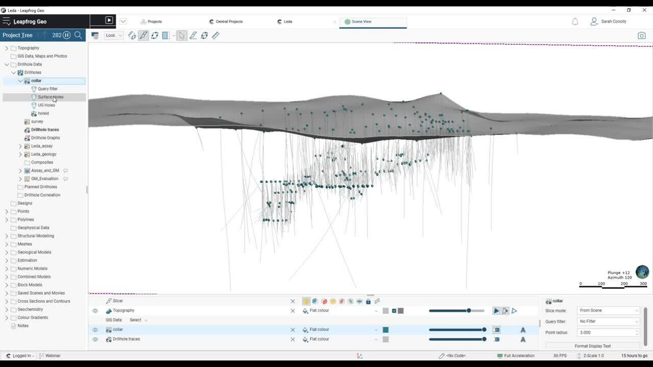
So here I am in Leapfrog Geo version six,

[00:14:12.660]
and as promised, it looks a little different.

[00:14:16.410]
However, we still have the Project Tree

[00:14:18.450]
on the left-hand side with all the folders that you used to.

[00:14:23.620]
The 3D scene in the middle, and our shape list

[00:14:29.470]
and properties panel down below.

[00:14:34.460]
The first feature that I’m going to demonstrate

[00:14:37.420]
within the software is the ability to project

[00:14:40.340]
a subset of colors onto the topography.

[00:14:44.703]
So you can see from this project

[00:14:46.370]
that I have both surface holes and underground holes

[00:14:52.290]
that were drilled once the mining had advanced.

[00:14:58.750]
Within my Drillhole data folder, under my color table

[00:15:04.570]
I’ve already created two query filters

[00:15:08.720]
to isolate my surface hole colors

[00:15:13.070]
from my underground hole colors.

[00:15:21.940]
If I want to project just my surface drill holes

[00:15:25.300]
onto this topography,

[00:15:26.990]
if I’m really confident that my pickup

[00:15:29.800]
is the more accurate data source,

[00:15:33.040]
then I can right click on the Color table,

[00:15:36.340]
head down the menu to Set Elevation,

[00:15:42.930]
and within this window, I get to select the query filter

[00:15:47.100]
that I want to subset my database on.

[00:15:49.950]
So I’m going to pick the surface holes.

[00:15:54.910]
From the surface, I get to select

[00:15:57.620]
what I would like to project the colors onto.

[00:16:01.100]
I’m going to pick my typography.

[00:16:04.490]
You can see that all the other surfaces within my project

[00:16:07.450]
are available in this list.

[00:16:10.050]
So it’s just a choice of what I use.

[00:16:13.860]
I’ll click “Okay.”

[00:16:15.660]
And this will reset any of the elevation

[00:16:19.260]
from my surface hole colors onto the topography

[00:16:24.040]
by altering the Z value.

[00:16:27.630]
Obviously this will then process

[00:16:29.070]
anything downstream within my project.

[00:16:33.830]
If I open up my Color table, you can now see

[00:16:37.790]
that not only do I have my X, Y and Z point for my color,

[00:16:43.780]
which is the original,

[00:16:45.590]
I also have a new column called Zed on terrain.

[00:16:50.400]
And you can see that there are slight changes

[00:16:52.780]
for some of my color points.

[00:16:57.610]
If for some reason I like to decide

[00:17:00.380]
that I don’t want to use that Z

[00:17:02.430]
that we’ve projected onto the topography,

[00:17:06.290]
I expand out the color elevation above the table

[00:17:10.750]
and I can always switch back to using the color elevation

[00:17:14.140]
from my original Z value.

[00:17:23.070]
So that is how you project a subset of data

[00:17:26.710]
onto a particular surface from your color table.

[00:17:34.520]
Next step I want to take a look

[00:17:36.240]
at my depth visualization in the 3D scene.

[00:17:41.700]
And I’ve isolated some data

[00:17:43.330]
so I’m only looking at small amounts of drilling.

[00:17:46.730]
I have my assets displayed,

[00:17:49.150]
and if I click on any of my intervals,

[00:17:52.290]
I’d like to draw your eye down to the data window

[00:17:55.120]
in the left-hand side, where you can now see

[00:17:58.530]
that we have an extra metadata called Downhole depth.

[00:18:04.350]
So depending on where you click on the drillhole,

[00:18:08.260]
the downhole depth will be displayed in this window,

[00:18:11.910]
along with the actual interval from and to as well.

[00:18:18.650]
If I’d actually like to be able to see

[00:18:20.470]
my downhole depth mark as well,

[00:18:23.800]
I need to head up to my Project Tree,

[00:18:26.320]
find the drillhole traces and load those into the scene.

[00:18:31.150]
I will apply the same query filter for these as well.

[00:18:37.710]
In order to display my depth marks in the properties panel

[00:18:41.860]
in the bottom right-hand corner,

[00:18:44.850]
I can tick on the Show Depth Marks,

[00:18:48.400]
and then I have some choices to make.

[00:18:51.430]
I get to decide how often I want to create a tick.

[00:18:55.640]
I’ll drop that down to every two meters,

[00:19:00.750]
how large I would like my tick width to be,

[00:19:06.400]
and how often I would like to label them.

[00:19:15.499]
You can dictate this in the window with the value,

[00:19:18.400]
but you do also need to show the text

[00:19:21.420]
within the Shape List objects as well.

[00:19:24.880]
So here, you can see I’ve labeled every 10 ticks.

[00:19:28.350]
I have my ticks for every two meters.

[00:19:30.600]
I get my depth mark at 20, 40, 60, et cetera, down the hole.

[00:19:40.080]
You can shift them to the left or the right-hand side,

[00:19:43.150]
and you can change the whole ID label as well.

[00:19:58.010]
Next, we’ll take a look at reloading our drilling

[00:20:01.050]
from the Central Data Room.

[00:20:03.680]
So we take a close look

[00:20:05.730]
at the drillhole tables in this project.

[00:20:08.290]
You can see that there’s a small C on each of the tables.

[00:20:13.220]
This shows that when the drill holes were first imported,

[00:20:16.920]
they were imported from the Central Data Room.

[00:20:21.290]
You may also notice that there is a small clock

[00:20:23.850]
on each of the tables.

[00:20:26.980]
This dictates that since I’ve been working on this project,

[00:20:31.692]
a new version of the CSVs for the drillholes

[00:20:36.730]
have been uploaded to the Central Data Room.

[00:20:41.270]
This has informed me now that my drilling has been updated.

[00:20:46.140]
Whenever I want to be working

[00:20:47.840]
from the most up-to-date version of my database,

[00:20:50.570]
I should reload the tables.

[00:20:54.040]
There are a few options here.

[00:20:56.380]
On individual tables, you can right click

[00:21:00.610]
and you can either decide to import the column

[00:21:03.360]
from the Latest File version,

[00:21:06.060]
or import the column from the File History.

[00:21:10.430]
When you pick this option, you can go to any version

[00:21:13.610]
that was published to the data room.

[00:21:18.100]
When you pick the Latest File version,

[00:21:20.230]
it will go to the very last version that was uploaded.

[00:21:27.320]
If I want to reload all of the tables at one go,

[00:21:30.640]
I can simply right click on the top level drillholes object

[00:21:34.910]
and reload the latest file versions.

[00:21:40.890]
This is then going to look to the Central Data Room,

[00:21:44.510]
see the new versions of the CSVs,

[00:21:47.240]
and I will then go through the process

[00:21:50.110]
of updating my drilling.

[00:21:52.340]
So you can still just check that the correct columns

[00:21:54.690]
have been imported and go from there.

[00:22:04.760]
The power of this workflow

[00:22:06.240]
comes when you’ve got a centralized data set,

[00:22:09.910]
but multiple people potentially working

[00:22:11.910]
on different projects from the same dataset.

[00:22:15.290]
You only need to update the Central Data Room one time

[00:22:19.700]
for all the people in their different projects

[00:22:22.480]
to see that there’s a new version

[00:22:25.080]
and that they can upload their local project.

[00:22:30.100]
This will take a few minutes to reprocess.

[00:22:40.550]
Now I’m going to demonstrate, well,

[00:22:42.710]
I think is the most exciting feature of this new release.

[00:22:46.200]
Calculations directly on drillhole tables.

[00:22:51.400]
In the same way just looking at my top hole obviously,

[00:22:54.890]
my drilling that’s been displayed

[00:22:56.440]
by my lithology from the login,

[00:22:59.340]
along with a couple of massive sulfide lenses

[00:23:02.960]
that have been modeled from the data.

[00:23:07.600]
If I want to create a calculation on any of my tables,

[00:23:11.280]
I right click on them in the Project Tree,

[00:23:14.170]
find the calculations in the menu,

[00:23:17.760]
and that will open this interface

[00:23:20.310]
where you can see that we have

[00:23:22.020]
our variables and calculations on the left,

[00:23:25.560]
a list of metadata and data from your drillhole table,

[00:23:33.980]
along with syntax and functions on the right hand side.

[00:23:38.710]
On my geology table,

[00:23:39.830]
I’m going to build a simple calculation

[00:23:42.600]
to use my geology as a proxy for my density.

[00:23:48.380]
So I’m going to create a new item

[00:23:51.490]
that the ability to create variables,

[00:23:53.730]
numeric and categorical calculations.

[00:23:57.490]
I’ll go for a numeric one today, and I’ll name this density.

[00:24:07.210]
And I really like to use these pick lists

[00:24:09.410]
on the right hand side to build my calculation.

[00:24:13.380]
And today I’m going to use a simple if statement

[00:24:18.890]
to say that if my lithology equals my LMS one,

[00:24:25.990]
my massive sulfide one, or, again,

[00:24:30.350]
I go to the syntax on the right hand side,

[00:24:33.880]
my lithology equals LMS two.

[00:24:38.190]
I’m going to give this a value of 4.5.

[00:24:41.630]
Otherwise I’ll set it at my background

[00:24:45.860]
density of around 2.7.

[00:24:49.500]
Once I click Save, that calculation will stall

[00:24:54.440]
within my geology table.

[00:24:58.260]
If I close that interphase,

[00:24:59.960]
and now I look to my 3D scene,

[00:25:03.560]
again, I’ll just hide those two volumes.

[00:25:07.630]
I can look to my geology table in the shape list

[00:25:11.850]
for the dropdown.

[00:25:13.590]
I can now display my drilling via the density.

[00:25:20.260]
And you can see that where I had

[00:25:21.640]
those two massive sulfide lenses,

[00:25:24.000]
which was based, modeled from my lithology,

[00:25:29.640]
I now have set the density values as 4.5.

[00:25:38.560]
So that’s one example of a calculation.

[00:25:43.700]
Another one that I’ll do on my essay table.

[00:25:46.980]
I’ll just remove a few things from the scene

[00:25:50.830]
and load in my essays, remove any filters.

[00:25:56.680]
If I’m going to create a calculation to display

[00:26:02.020]
my gram meters for my gold values.

[00:26:05.330]
So again, I right click on the table, find my calculations,

[00:26:11.560]
and then this will open up my calculations

[00:26:14.760]
from my essay table.

[00:26:17.210]
So you can see I’ve actually

[00:26:18.140]
already got a few things loaded in here.

[00:26:21.240]
I’ve got some variables that are defining

[00:26:23.730]
the current price of silver as zinc and lead.

[00:26:27.670]
I’ve created some factors between my different metals,

[00:26:33.270]
and then I’ve used these variables

[00:26:35.110]
in a zinc equivalency calculation

[00:26:38.310]
to combine the different metals

[00:26:40.280]
that I’m interested in in this deposit.

[00:26:48.400]
I’ll create the new calculation now,

[00:26:50.560]
which again, is just going to be a new item,

[00:26:54.040]
a numeric calculation.

[00:26:55.870]
This time I’m going to calculate my gram meters,

[00:27:04.548]
click “Okay” and this one’s going to be even more simple.

[00:27:09.320]
I’m going to go to my main metadata list.

[00:27:14.360]
I’m going to grab my into the length

[00:27:16.740]
and multiply that directly by my gold value.

[00:27:21.720]
Length times grade and I’ve got my ground meters

[00:27:26.010]
for that drill hole interval

[00:27:30.520]
I’ll click Save,

[00:27:32.090]
and the same idea can be applied in the 3D scene.

[00:27:35.140]
So I go back to my Scene View

[00:27:37.860]
Now on my drop down,

[00:27:39.600]
I have my original elements that were assayed,

[00:27:42.760]
but I can also display my drilling by the gram meters,

[00:27:48.680]
or in fact that zinc equivalency calculation

[00:27:51.070]
that I already prepared and advanced.

[00:27:56.610]
Other examples of calculations that could be used include

[00:28:00.450]
element ratios for geochemical analysis.

[00:28:04.110]
So the metal equivalency calculations

[00:28:06.140]
depending on your deposit or creating top cap grade

[00:28:10.260]
variables for statistical analysis.

[00:28:13.940]
I’m sure you guys have lots of other ideas.

[00:28:15.900]
So maybe throw into the questions of some of the things

[00:28:20.010]
that you think you could potentially use this tool for.

[00:28:25.470]
Now we will take a look at the improved mesh error

[00:28:28.500]
visualization ability in Leapfrog.

[00:28:33.370]
In the scene I have a mesh that I have imported

[00:28:36.250]
from another software package.

[00:28:39.300]
In the projectory,

[00:28:40.640]
you can see that this mesh has been loaded

[00:28:42.960]
and we have the small exclamation mark

[00:28:45.740]
suggesting that there was an issue with the mesh.

[00:28:50.110]
Rather than having to right click and go to properties,

[00:28:52.720]
now if you expand the object,

[00:28:54.680]
you’ll see the issue sitting beneath it.

[00:28:57.710]
And in this example,

[00:28:58.940]
you can see that we have some self intersections.

[00:29:03.560]
I can load the self intersections in the scene

[00:29:06.500]
and it will be its own object.

[00:29:09.730]
I’ve already made it a nice bright color

[00:29:12.000]
by clicking on the little color swatch

[00:29:14.570]
and selecting something really bright.

[00:29:20.070]
To locate it, you can do a few things,

[00:29:22.090]
you could hide your original mesh.

[00:29:27.170]
You may wish to make your mesh translucent

[00:29:30.930]
say that you can kind of spin it around

[00:29:32.760]
and see where they’re located.

[00:29:35.860]
Or sometimes I prefer to just show the edges

[00:29:38.860]
and turn off the triangle faces.

[00:29:42.870]
And then it’s really obvious where those triangles are,

[00:29:45.870]
that’s our intersecting.

[00:29:49.330]
So you can’t necessarily fix these in Leapfrog.

[00:29:53.290]
However, if you right click and export,

[00:29:56.540]
you can export these as a number of different file types

[00:30:01.860]
in order to go back to the original software

[00:30:04.550]
and tweak the mesh within that.

[00:30:11.960]
I have another mesh within here,

[00:30:14.830]
that I’d like to load the fault zone,

[00:30:17.440]
and I’m going to expand out the object beneath it.

[00:30:22.160]
So there’s no actual error associated with this fault.

[00:30:26.810]
You can see that I have my broader edges

[00:30:29.560]
and my non-manifold edges.

[00:30:32.060]
So we do have some non-manifold edges.

[00:30:34.720]
However, this mesh is now allowed to continue on

[00:30:38.810]
down the workflow in Leapfrog.

[00:30:43.960]
If I want to visualize where these issues are all,

[00:30:50.970]
I can drag them into the scene

[00:30:52.800]
and you can see that the border edge

[00:30:54.930]
is simply a line around the margin of our mesh.

[00:31:00.450]
If I hide the mesh itself, you can see it more clearly.

[00:31:06.240]
If this mesh was actually missing a few triangles

[00:31:09.310]
and had any holes on the inside, we would also see

[00:31:12.690]
those being displayed in the scene from this feature.

[00:31:20.770]
For my non-manifold edges,

[00:31:22.350]
I can also drag those into the scene.

[00:31:25.910]
It’s been my model around and take a look

[00:31:28.760]
to see where those issues lie.

[00:31:31.440]
And again, I can use a different visualization tools

[00:31:35.180]
in order to zone in on the area I need to fix.

[00:31:42.270]
Remember any of these objects,

[00:31:44.150]
you can right click on them in the Project Tree X-Box

[00:31:48.040]
to take a look elsewhere.

[00:31:53.580]
Onto a simple one here,

[00:31:56.190]
which you’ve been asking for awhile,

[00:31:59.650]
which is reordering legends.

[00:32:02.070]
Here, I have my lithology table

[00:32:04.370]
and I want to list the legend in a different order.

[00:32:09.783]
I’ve got my drilling displayed and you can see my legend

[00:32:12.370]
in the top right hand corner.

[00:32:16.910]
All I need to do to reorder them

[00:32:18.900]
is to head down to the Shape List, click on my Edit colors,

[00:32:24.650]
and now along with being able to turn on

[00:32:27.200]
and off individual lithologies,

[00:32:30.140]
we can reorder them using the up and down arrows

[00:32:34.010]
on the right hand side.

[00:32:37.770]
So I can focus in on the lithologies that matter.

[00:32:46.180]
This can also be done within geological models

[00:32:49.730]
or anything else that you have a legend associated with it.

[00:32:54.940]
So if I just quickly clear my scene

[00:32:59.380]
I’m going to head down to bi-combined model,

[00:33:02.350]
and I’ve got a pick depletion model,

[00:33:06.140]
where I have my two massive sulfide lenses

[00:33:08.400]
coded by potential stage one stage two pits.

[00:33:14.580]
But you can see that my legend

[00:33:15.780]
is all over the place in the top right hand corner.

[00:33:19.350]
So again, all I need to do is edit colors

[00:33:22.580]
and just think a little bit about my legend over here.

[00:33:29.870]
So I’m going to do my LMS one stage one and two,

[00:33:34.231]
my LMS stage two, the one and two,

[00:33:39.130]
and then my two domains outside of the pit.

[00:33:47.200]
Last but not least, I’m going to show you the thing

[00:33:49.970]
that I think is the second most exciting thing

[00:33:52.940]
about this Geo release.

[00:33:56.030]
And that’s the ability to be able to import

[00:33:59.225]
a full geological model from another central project

[00:34:03.450]
into the project you’re working in.

[00:34:06.820]
Many users currently import output volumes

[00:34:09.860]
from a geological model produced in another Leapfrog project

[00:34:13.610]
as a mesh into the meshes folder.

[00:34:17.510]
This then requires the model to be rebuilt

[00:34:19.980]
within this current project.

[00:34:24.270]
With this latest release of Geo and central,

[00:34:27.240]
you’ll now be able to import full geological models

[00:34:30.450]
directly into the geological models folder.

[00:34:34.950]
These models will be static.

[00:34:37.630]
However, you can definitely use them

[00:34:40.170]
for downstream processes.

[00:34:42.020]
For example, if you evaluate them onto your drillholes

[00:34:45.453]
and you’re doing some EDA,

[00:34:48.190]
or you could use the output volumes

[00:34:49.730]
of these imported geological models

[00:34:52.200]
after means for resource estimation.

[00:34:58.700]
The process room part in these models is fairly simple.

[00:35:03.640]
As long as you’re connected to central,

[00:35:06.930]
you can right click on the geological models folder,

[00:35:10.590]
import the geological model from central,

[00:35:14.530]
and then look to your other projects

[00:35:18.090]
that you want to grab the model from.

[00:35:20.840]
In my case, I’m going to use the leader exploration project.

[00:35:28.130]
For this example, I’m going to import what we call

[00:35:30.340]
the upper Ms. geological model.

[00:35:34.920]
So I select it on the right hand side, click Import.

[00:35:42.370]
This project will look to central, import this model,

[00:35:46.100]
and you can see that I have a new model in my Project Tree.

[00:35:50.340]
If I drag this into the scene,

[00:35:52.550]
you can see it’s only for half of the data.

[00:35:57.900]
However, this is one of the branches

[00:36:00.580]
that one of my teams has been working on.

[00:36:03.000]
And then someone else would actually

[00:36:04.600]
working on the lower zone, which I could import as well.

[00:36:08.860]
One thing I like to show

[00:36:10.810]
is if I expand these out in the project tree,

[00:36:13.010]
you can see the boundary default system,

[00:36:15.930]
the surface chronology.

[00:36:18.530]
However, if I right click on any of the surfaces

[00:36:20.960]
under the surface chronology, they can’t be edited.

[00:36:24.290]
As I mentioned,

[00:36:25.350]
that needs to happen in the original projects.

[00:36:30.660]
If my colleagues that were working on this model updated

[00:36:34.350]
and republished a new version of this model,

[00:36:37.690]
similar to my drillhole data,

[00:36:39.410]
I would get the small clock on the geological model.

[00:36:43.600]
And it would tell me

[00:36:44.433]
that there’s a new version of this model

[00:36:46.560]
and do I want to reload the latest on that branch?

[00:37:01.980]
So with that, I’d like to thank you for joining me today.

[00:37:06.080]
Please, as I mentioned,

[00:37:07.770]
ask any questions that you have in the window,

[00:37:11.370]
and we will endeavor to get back to you

[00:37:13.430]
on any of your questions as soon as possible.

[00:37:17.280]
If something pops up later on,

[00:37:19.880]
or you watch the recording rather than see this live,

[00:37:23.020]
then do feel free to reach out to [email protected].

[00:37:28.550]
And we’ll put you in touch

[00:37:29.850]
with someone from our technical team

[00:37:32.160]
to discuss any of your questions or queries.

[00:37:36.160]
Thank you and I hope that you enjoy the new release.