


Classical geostatistical estimation requires the user to define volumes of stationarity (domains) within which estimation can be safely performed. In basic estimation a single constant orientation for search and variogram is then applied across the domain. If the geometry of the domain, and the mineralisation within, is very planar using a single global orientation may be appropriate but if the domain is more typical and undulates, then use of the global search may locally result in sub-optimal sample selection and/or sample weighting.
Leapfrog Edge’s Variable Orientation (VO) tool overcomes this problem by allowing the user to locally re-orientate the search and variogram during estimation to better match the local geometry.
The workflow to create and apply a VO will be obvious and intuitive for Leapfrog users, with the usual strong focus on clean design, considered functionality and contextual 3D visualisation.
Use
The Variable Orientation feature has been designed and implemented with a specific purpose or use case in mind. For narrow tabular domains, such as veins or stratigraphic surfaces, even minor changes in orientation of the surface can greatly impact the local selection of samples, and the weighting given those samples in estimation. One solution to this irregularity is to break the domain up in to sub-domains of different orientation, but this is time consuming and introduces artificial internal boundaries. A better alternative, the solution we have implemented in Variable Orientation, is to re-orientate the search and variogram locally, so that the principal orthogonal plane (the plane containing major and intermediate axes) matches the local geometry. In essence, each cell of the block model becomes its own local sub-domain.
The Variable Orientation object has two inputs: a mesh (or meshes) and a global plunge. The global plunge can be defined from either a ‘global’ variogram (i.e. a variogram defined on all data in the domain with an ‘average’ orientation or from a global plunge vector that can be set from the viewer (or manually typed in). A unique feature of the variable orientation tool is that it preserves the global plunge in the locally re-orientated ellipsoid.
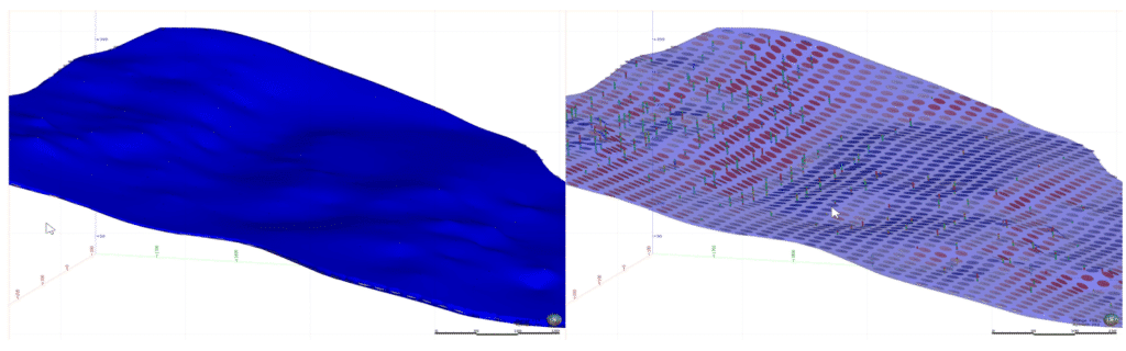
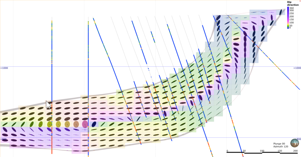
In keeping with Leapfrog’s ethos, we have made the VO tool highly visual, so the user can clearly understand the impact of applying variable orientation and visualise this in relation to the target domain, available sampling and any other object in the 3D scene. In the setup of the visualisation of the variable orientation, the user specifies whether to visualise onto an existing block model or on to a customised grid. Once processed, the variable orientation object can be dragged into the scene where the re-oriented principal planes (i.e. the plane containing major and intermediate axes) can be visualised as a re-sizeable disk or as an ellipse that reflects the anisotropic ratio of the major/intermediate axes. Disks can be coloured by dip or dip direction. If the scene is too crowded, the disks can be turned off, and the vector of the re-oriented major axis shown instead. [For those who use the structural trends, this is the visualisation that you wished that object had! Watch this space.]
Pro Tips
When you want to visualise or create presentation materials for a narrow structure, use a variable Z sub-block model, with a single block in Z and sub-blocks triggered on the domain of interest. The evaluation will create a single layer of disks on the interval mid-plane.
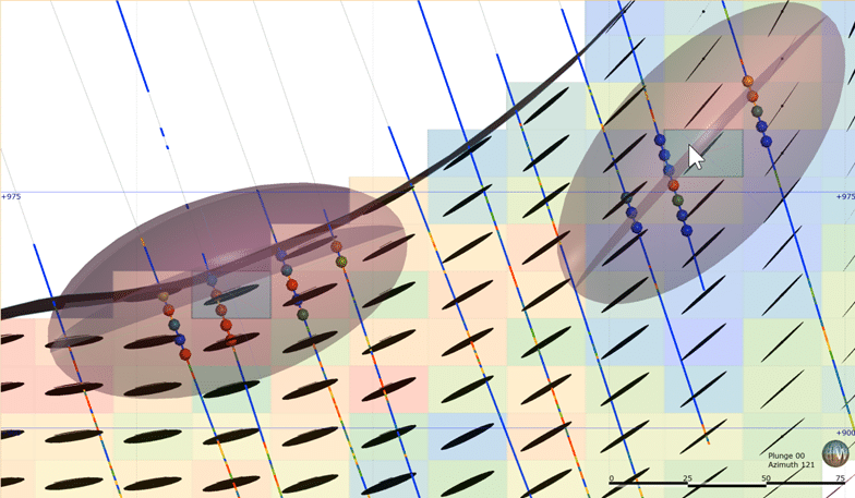
While the visualisation of the VO across the domain is invaluable for validating the relationship between input meshes and the output orientations, this is only part of the story. We have also coupled the VO with the ‘block interrogation’ tool, so the user can visualise the locally oriented search ellipsoid and the effect that has on sample selection, simply by clicking on any block in the domain. Cool eh!
It really
is as simple as that.
Like all of
Leapfrog’s tools, we have strived to make the use and utility of VO as simple
and intuitive as possible. But of course, there is sophisticated, well tested, robust
mathematics going on in the background. None of this is a secret, we just
believe the user shouldn’t have to be exposed to irrelevant detail, just focus
on the task at hand.
That said, we think it is helpful to know a little of how this works in order to understand how to use the tool most effectively.
A little background
The Variable Orientation tool uses mesh inputs to control the local orientation. The variable orientation is calculated from the vertices of an input mesh (or meshes). Normal vectors are calculated at each vertex, then decomposed into three orthogonal vectors which are interpolated independently using RBF’s. This allows the local orientation of the normal vector, and the principal plane perpendicular to this, to be reconstructed at any location. A few implications from this approach that you should be cognisant of:
1) The effort/time in creating the VO object is dependent on the number of vertices in the input meshes. Be careful to ensure that the input meshes have an appropriate resolution to capture local variability in orientation, but do not contain irrelevant detail as this will slow down processing.
2) The facing direction of the mesh is important, as calculation of the normal vector takes facing into account. When using 2 or more meshes, the facing directions need to be complementary. For Vein and Stratigraphy objects, we know the facing directions, and so can automatically ensure that surface facing is consistent. When using other mesh inputs it is up to the user to check consistency – the easiest way to do this is by visualisation in scene.
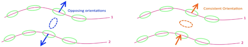
3) Closed meshes should only be used as input to VO with great caution. Because the vector field is directional, a closed mesh will produce indeterminate results at the midpoint, when the vector contributions from either side will be in opposite directions. This is immediately obvious when the VO is viewed in scene.
Early adopters have asked what the ‘global plunge’ represents.
The local re-orientation is based on interpolation of the normal vector. The plane perpendicular to the normal contains the major and intermediate axes. The question is, where should the principal and intermediate axes lie in the re-oriented principal plane. We answer this question by projecting the ‘global plunge’ vector on to the new principal plane – imagine a spot light shining perpendicular to the principal plane along the re-oriented normal vector – the new major axis position is the shadow cast by the global plunge vector. Not coincidentally, this orientation is also where the angular difference between the ‘global plunge’ vector and the new major axis is minimised. Once we have located the new major axis, then the intermediate axis simply lies 90° away in the principal plane.
Get more from Leapfrog Edge – talk to an expert today.