Leapfrog Edge 4.0 – Take a tour of the new Parameter Report and more

This webinar is the best place to learn how the new functionality can improve efficiency in your workflows, give you more flexibility and help you make decisions faster.

Webinar highlights include:

• Estimation management with the new Parameter Report
• Additional economic compositing options
• Lock total sill in variogram modelling
• New variogram model types
• Explore the new interface
• And much more!

Video Transcript

[00:00:01.600]<v Instructor>Welcome to the release webinar</v>

[00:00:03.380]for Leapfrog Geo version 6.0.1

[00:00:06.700]and Edge Extension version 4.0.1.

[00:00:11.210]Please note, we have released these updated versions

[00:00:14.500]as we identified an issue which may have prevented you

[00:00:17.490]from accessing the new version of the software.

[00:00:20.760]We want to deliver a great user experience

[00:00:23.430]and are pleased to say, this is now fixed,

[00:00:26.190]and the new release is ready for you to download.

[00:00:30.130]This new release is a big one for Seequent,

[00:00:32.730]Leapfrog not only looks different,

[00:00:34.900]but has some key features that many customers

[00:00:37.130]have been asking for.

[00:00:39.180]But before we get going,

[00:00:40.590]there are a couple of go-to meeting logistics.

[00:00:43.690]If you take a look at the go-to webinar dialogue panel,

[00:00:46.800]you should see a place for questions.

[00:00:49.080]Can you take a moment to type yes if you can hear me?

[00:00:53.430]I won’t be answering questions during the webinar,

[00:00:56.020]so please use this panel to enter your questions

[00:00:59.060]and I will answer them with a personal email

[00:01:01.750]after the webinar ends.

[00:01:04.700]Here is an overview of the main themes we will be discussing

[00:01:07.510]in this product update.

[00:01:09.540]I will introduce some of them here,

[00:01:11.610]and describe them in more detail later in the webinar.

[00:01:15.390]We have a new user interface,

[00:01:18.940]improvements to drillholes,

[00:01:21.700]better mesh handling, estimation parameter management,

[00:01:26.890]block model reporting improvements, and more.

[00:01:31.910]The you Leapfrog user interface is the first thing

[00:01:34.390]we want to talk about because there is no escaping

[00:01:37.120]the fact that it looks different to the last release.

[00:01:40.920]Seequent has put a huge amount of effort into updating

[00:01:43.800]the building blocks of Leapfrog, and this has enabled us

[00:01:46.940]to introduce a new user experience.

[00:01:51.160]The new user interface of Leapfrog is sleek, streamlined,

[00:01:55.490]and brings cohesion

[00:01:56.560]across the Seequent portfolio of products.

[00:01:59.920]While it may appear quite different at first glance,

[00:02:02.770]all of the functionality remains in exactly the same place

[00:02:06.290]as it was before.

[00:02:08.890]Secondly, we wanted to show you the effort we have put

[00:02:11.680]into making your Leapfrog experience better

[00:02:14.240]when using some of the main functionality.

[00:02:17.000]We have made improvements to the drillhole database

[00:02:19.740]so that your modeling is based on quick to load, accurate

[00:02:23.260]and easy to update data.

[00:02:26.740]We’ve made improvements to the processing of tasks

[00:02:29.360]in parallel so that your drilling data can process

[00:02:33.300]and reload substantially quicker for some projects.

[00:02:36.610]In some instances, we have reduced the processing time

[00:02:40.090]by over 40%.

[00:02:43.150]To make importing drilling data easier,

[00:02:45.470]you can now import your downhole points

[00:02:47.640]from structural data for instance,

[00:02:49.870]at the same time as your collar, survey,

[00:02:52.150]and interval tables.

[00:02:54.860]Made a mistake when importing,

[00:02:56.590]or no longer require one of your data columns?

[00:02:59.730]Leapfrog will now allow you to rename

[00:03:02.280]and delete your imported columns.

[00:03:04.810]This will enable you to keep your data

[00:03:06.800]up to date and relevant.

[00:03:09.530]This option is available for all data tables,

[00:03:12.250]including collars, interval tables, GIS,

[00:03:15.800]and structural data.

[00:03:18.510]And now what we think is the most exciting addition

[00:03:20.850]to the drillholes, calculations.

[00:03:24.140]Use this tab to write calculations

[00:03:26.160]that will categorize, combine or reclassify your data.

[00:03:30.730]You can for instance, add a new calculated column

[00:03:33.460]for capped assay values prior to compositing.

[00:03:37.460]Calculations are also available for calculated points

[00:03:41.000]such as mid points, guide points and grade of points.

[00:03:46.090]Dealing with invalid measures can be problematic,

[00:03:49.080]it is often hard to locate

[00:03:50.470]where the problems are to fix them,

[00:03:52.320]we have made some changes in this release

[00:03:54.200]to make this easier.

[00:03:56.550]Firstly, we have improved the way we categorize

[00:03:59.540]the mesh issues.

[00:04:01.100]It is now clear which errors the mesh contains

[00:04:03.840]from the tree view directly,

[00:04:06.000]instead of having to look at the properties of the mesh.

[00:04:10.000]Secondly, the tickbox to view the border edge on a mesh

[00:04:13.540]has now been turned into its own separate object.

[00:04:16.870]This means you can view the location

[00:04:19.830]of the issue in the scene independent of the mesh.

[00:04:23.460]In addition, the border edges object can be exported

[00:04:26.860]as a polyline file, which can be visualized

[00:04:29.950]in the source software of the mesh.

[00:04:33.110]We have also added another categorization to the way

[00:04:36.270]we define non-manifold meshes,

[00:04:39.560]as well as being able to view the non=manifold edges

[00:04:42.300]in the scene as their own object.

[00:04:44.440]We have also enabled some non manifold meshes to be used

[00:04:47.860]that were once unusable.

[00:04:50.750]Non-manifold meshes with an even number

[00:04:53.100]of adjoining triangles are now usable.

[00:04:56.240]However, non manifold meshes with an odd number

[00:04:59.140]of adjoining triangles will result

[00:05:01.170]in an object named odd non-manifold edges,

[00:05:04.860]and these will remain unusable.

[00:05:08.030]For more information on the improvements in Geo,

[00:05:10.520]please watch the Leapfrog Geo version 6.0.1 release webinar

[00:05:14.580]and video.

[00:05:16.810]And now a highly requested new feature for block estimation.

[00:05:21.320]Leapfrog has developed the estimation parameter report

[00:05:25.000]to help make multi-domain estimation more efficient.

[00:05:30.020]This is the first step in an initiative to describe,

[00:05:33.590]to transform the creation and management

[00:05:35.740]of resource estimation parameters in Edge.

[00:05:39.510]The parameter report allows you to view

[00:05:41.760]the estimation parameters for every estimator

[00:05:44.410]in your project.

[00:05:46.600]Use the domain and filters to refine your parameter view.

[00:05:50.920]Swap between tabs to change your parameters.

[00:05:54.340]Click in the sill to open the relevant object for editing.

[00:05:57.960]Click on the headers to sort the rows

[00:05:59.670]to identify patterns or errors.

[00:06:02.270]Use the export button to export your parameters

[00:06:05.030]to an Excel spreadsheet.

[00:06:06.770]Regardless of your filtering, the entire parameter report

[00:06:10.080]will export to allow for filtering in Excel.

[00:06:13.670]Tabs and the parameter report will be displayed

[00:06:16.280]in different worksheets in Excel.

[00:06:19.280]In this release, we have tried to identify some improvements

[00:06:22.120]that will make your estimation easier.

[00:06:25.320]We have made improvements to the variogram tab

[00:06:28.050]to help you with your variography.

[00:06:30.690]Firstly based on feedback,

[00:06:33.000]we have added the option to lock the total sill,

[00:06:36.670]click on the padlock to lock the total sill.

[00:06:39.370]Changes made to the structures will no longer affect

[00:06:42.030]the total sill, this is especially useful

[00:06:45.120]for fitting variograms with two structures.

[00:06:48.360]We have also added four more variogram model types

[00:06:51.730]to provide additional flexibility when modeling variables,

[00:06:55.380]which have high continuity and high local correlation.

[00:06:59.900]The exponential model, which is steeper at the origin

[00:07:02.580]than the spherical or spheroidal model

[00:07:04.750]and is commonly used for metals.

[00:07:07.090]Gaussian, cubic, and generalized Cauchy,

[00:07:09.990]which are more continuous near the origin.

[00:07:13.670]Here are some usability improvements that we think will help

[00:07:16.280]you when creating your estimation project.

[00:07:19.960]When creating a numeric composite within a subset of codes,

[00:07:23.370]we have now added the resulting lithology column

[00:07:25.820]from the base column used.

[00:07:28.270]This means that your numeric composite table

[00:07:30.880]is already merged with the base column,

[00:07:33.560]reducing the need to make merge tables,

[00:07:36.090]to combine your numeric composite

[00:07:37.910]with your lithology domain.

[00:07:40.280]With large block models it can be difficult to use

[00:07:43.150]the index filter to capture the blocks

[00:07:45.090]you want to visualize.

[00:07:46.820]We have added an extra control to allow you to zoom

[00:07:49.980]into the filter range and refine it further.

[00:07:53.140]This feature is used in block visualization

[00:07:55.840]and in swath plots.

[00:07:58.280]Lastly, we have made some improvements

[00:08:00.070]to block model reporting to make it more flexible

[00:08:03.300]for different types of resources.

[00:08:05.820]The ability to report below the cutoff is helpful

[00:08:09.700]for those reporting on industrial minerals or contaminants.

[00:08:13.710]We have added carats as a reporting unit for those looking

[00:08:16.630]to estimate diamond resources.

[00:08:19.190]And for those looking to create a great tonnage report,

[00:08:22.570]we have also added the ability to report below the cutoff.

[00:08:26.610]This will invert the grade tonnage curve.

[00:08:30.040]I will now demonstrate some of the new features

[00:08:32.100]in Leapfrog Edge version 4.0.1.

[00:08:36.560]The first new feature I’d like to show you

[00:08:38.710]is the improvement in numeric compositing.

[00:08:42.570]So we have the Leda training project here.

[00:08:45.650]Those of you who have taken training from us

[00:08:48.040]will recognize it immediately.

[00:08:50.010]Now I’m going to right click on composites,

[00:08:53.100]select a new numeric composite

[00:08:55.980]using a subset of codes ’cause I want to see the lithology.

[00:09:00.500]The base column will come

[00:09:01.680]from the geological model evaluated

[00:09:04.710]onto the drillhole traces.

[00:09:07.410]And we’ll select a logical compositing length,

[00:09:12.620]two meters in this case, with a minimum coverage

[00:09:15.340]of 0% so that every interval has a chance

[00:09:19.030]of becoming a valid composite.

[00:09:21.470]And for short length composites,

[00:09:25.320]if there’s a residual length less than a meter,

[00:09:27.860]we will distribute it equally amongst

[00:09:31.296]all of the composites in the interval.

[00:09:34.450]And we’ll just give this a nice name call it the numb comp,

[00:09:39.360]I like to shorten it a little bit, two meters.

[00:09:43.410]And the output columns we will grab

[00:09:46.130]all of our Leda assay columns,

[00:09:50.700]and then click okay.

[00:09:53.770]So we’ll see that the structure of the table

[00:09:56.290]is already there.

[00:09:57.930]And you’ll notice that the GM,

[00:10:00.960]the geological model evaluation is there as a column,

[00:10:06.620]where previously we would have had to do

[00:10:09.730]a separate merge table and combine the assays

[00:10:14.320]with the GM evaluation, so that’s processed.

[00:10:18.780]Let’s how the look at the GM, there it is.

[00:10:23.610]Flat traces we can make them rendered tubes,

[00:10:29.370]a three meter radius,

[00:10:31.800]and we can also look at our composited zinc here

[00:10:36.180]just to check.

[00:10:37.013]So those are all two meter composites.

[00:10:41.230]The next new feature I’d like to show you

[00:10:43.410]are drillhole calculations.

[00:10:45.350]I think this is an important one

[00:10:46.700]that you’re going to appreciate.

[00:10:48.210]So let’s say for instance we want to add a capped column

[00:10:52.000]to an assay table.

[00:10:54.750]So here we have our Leda assays.

[00:10:57.120]We can look at our silver,

[00:10:58.650]I believe there are some outliers in silver,

[00:11:01.210]and just have a look at the unit various statistics.

[00:11:03.770]So here’s a log probability plot of silver,

[00:11:07.100]and it does look like there could be a tail here

[00:11:09.770]at two, three, four, five,

[00:11:11.820]above 500 perhaps around 600 grams per ton.

[00:11:16.030]We can look at the histogram.

[00:11:18.520]And we can see that similarly there’s the tail there,

[00:11:21.360]so without further analysis, let’s choose 600 grams

[00:11:26.600]as a reasonable capping value.

[00:11:30.130]So then we go to our Leda assay table,

[00:11:33.300]right click and select calculations.

[00:11:36.690]And we get the same calculations and filters panel that

[00:11:41.010]was available for block modeling and for points

[00:11:44.470]in the most recent release.

[00:11:46.150]Now I’m going to add

[00:11:47.140]a new numeric calculation.

[00:11:51.270]Going to call it a Ag Cap,

[00:11:56.010]click okay and then write a short if statement,

[00:12:01.450]if my silver

[00:12:05.120]is greater than 600,

[00:12:11.360]then the result is capped at 600.

[00:12:16.000]Otherwise it will get the silver value,

[00:12:20.700]no errors I’ll click save.

[00:12:23.670]And as it is saved,

[00:12:27.500]it is computed and it’s there now

[00:12:30.813]under calculations.

[00:12:32.440]These are the imported columns and the Ag Cap

[00:12:35.980]is there as a calculated column.

[00:12:39.270]Let’s just remove our numeric comp

[00:12:43.930]and then bring in the capped silver.

[00:12:47.890]And there’s the cap silver and of course you can select

[00:12:52.200]any of the other columns in the table from the dropdown.

[00:12:55.260]So there is capped and uncapped,

[00:12:59.020]go back to the capped and let’s have a look

[00:13:01.560]at the unit various statistics on that capped value.

[00:13:06.140]So we’ll have a look at the histogram of the log

[00:13:09.380]and there we can see our maximum value capped at 600

[00:13:13.470]so there is a new calculated column.

[00:13:17.770]The next thing we’ll have a look at are some

[00:13:19.900]of the mesh issues that we were talking about earlier.

[00:13:23.400]So let’s just clear the scene

[00:13:26.310]and collapse the project tree

[00:13:29.170]so that we can find things better.

[00:13:30.800]And here’s the meshes,

[00:13:32.600]and here we have meshes with issues.

[00:13:36.950]So here is a mesh with

[00:13:39.783]just we can look at the border edges.

[00:13:43.450]So there are the border edges.

[00:13:46.450]And in this case, we’ll just get that mesh into the scene.

[00:13:49.500]Now we can see that mesh

[00:13:52.880]has a hole in it identified by the mesh edge

[00:13:57.770]and if we want to repair this in another software,

[00:14:01.710]the source software we can right click and export that

[00:14:05.900]as a polyline, so a Leapfrog polyline file

[00:14:08.970]or any of the other supported exchange formats.

[00:14:13.730]DXF for instance,

[00:14:17.810]I will just clear these.

[00:14:21.090]And we have another issue here.

[00:14:24.250]Here we have a fault zone

[00:14:28.660]and there are some mesh issues showing up here somewhere.

[00:14:34.630]Let’s just hide that overall

[00:14:36.360]So there are still some remaining problems

[00:14:41.270]and it’s showing us where

[00:14:44.685]we can now export these and send them back for repair.

[00:14:51.140]Let’s get rid of these and have a look

[00:14:54.160]at the fault zone mesh, there’s an issues here as well.

[00:14:59.160]There’s our fault so a mesh,

[00:15:02.190]and we have still some non-manifold edges

[00:15:07.090]that need to be addressed.

[00:15:08.980]And they’re just very, very small objects

[00:15:13.480]in that mesh.

[00:15:15.280]But now we can export those non manifold edges,

[00:15:21.630]again as any one of the supported file formats.

[00:15:25.990]And we could perhaps fix these in the source software

[00:15:31.780]where the mesh came from.

[00:15:35.898]The next new feature I’ll show you is the ability

[00:15:38.630]to lock the total sill in the variogram.

[00:15:41.360]So let’s remove our meshes which is collapsed meshes,

[00:15:46.340]go down to the estimation folder

[00:15:49.270]and let’s have a look at zinc in the domain MLS1.

[00:15:54.280]Spatial models is where our variograms are,

[00:15:56.740]we have some already built here as the variogram model

[00:16:01.280]for zinc in LMS1.

[00:16:05.330]The opening page always shows us

[00:16:07.017]the three nested variograms.

[00:16:09.900]And if we look at the radial plot,

[00:16:12.240]we can see the orientation

[00:16:14.480]of our experimental models

[00:16:18.300]and experiment variogram and models.

[00:16:21.060]And let’s go now to the major access tab.

[00:16:24.510]This one has already been reasonably modeled

[00:16:28.850]or modeled reasonably well.

[00:16:32.320]And what I’ll show you is that here is the lock

[00:16:35.150]that we can use that will enable

[00:16:38.460]the total sill to remain fixed.

[00:16:41.170]So currently I can move my sill around

[00:16:44.740]and it is free as I changed the range,

[00:16:49.360]perhaps I could inadvertently alter my model.

[00:16:53.520]So I think I’ll just go back to set this

[00:16:58.630]to be 0.3, the second structure 0.3,

[00:17:01.960]so that my three models now sum to one.

[00:17:06.240]I want to put that handle back into its position here

[00:17:12.090]out to the maximum range there.

[00:17:13.940]So I’m going to click on the lock.

[00:17:16.560]And now when I drag that handle,

[00:17:19.870]it is not changing the gamma values.

[00:17:24.070]I can just put it into position

[00:17:26.370]and let’s just make that to be 160 meters full stop.

[00:17:32.590]This is a good opportunity to show you as well

[00:17:37.145]the four new model types that we’ve added.

[00:17:40.180]Perhaps we can close this one and add a new variogram

[00:17:43.840]I’ll just discard any changes that we made there,

[00:17:48.090]and go down to our spatial models

[00:17:50.380]and select new variogram model.

[00:17:56.430]And go to the access aligned variograms let’s set.

[00:18:02.840]Well, we need to put in a reasonable Dip

[00:18:05.370]for our LMS1

[00:18:09.780]Dip Azimuth.

[00:18:11.700]I can remember these values pretty well.

[00:18:19.975]We’ll just look at the one structure

[00:18:21.700]or a model with one structure so we can see what

[00:18:25.440]the shape of these curves looked like

[00:18:27.000]when we changed the different model types.

[00:18:30.930]So we have our spherical model

[00:18:34.920]and spheroidals, you’ll recognize those.

[00:18:38.550]And you’ll see that a portion of the model is linear

[00:18:43.060]before it starts to rise to the sill.

[00:18:46.490]And if we look at the exponential

[00:18:48.710]now it is steeper near the origin.

[00:18:50.830]There really isn’t a linear portion of the curve any longer.

[00:18:55.270]This does suit metals quite well

[00:18:58.790]like silver, gold, even the zinc.

[00:19:02.530]If we look at our lag distance here,

[00:19:05.640]I’ll just increase it to be 15.

[00:19:09.510]We can see now that the curve

[00:19:11.780]is approaching the sill,

[00:19:15.490]I can move that.

[00:19:19.720]Let’s just lock the sill.

[00:19:25.100]It looks like I’ll need another structure to model that,

[00:19:27.410]but I’m capturing the close range continuity

[00:19:31.680]a little bit better.

[00:19:33.730]Now, some of the other models here is the Gaussian,

[00:19:37.280]you’ll see that it is showing

[00:19:39.860]much better continuity near the origin,

[00:19:43.900]similarly cubic, slightly different shapes

[00:19:47.910]in the generalized Cauchy.

[00:19:50.351]With these models of course,

[00:19:52.850]if you’re estimating metals,

[00:19:54.400]you may find that it creates a bit of a smoothing

[00:19:58.490]near the blocks.

[00:20:01.580]This is introduced really

[00:20:04.270]for contaminants and things like that.

[00:20:07.070]So I think we can close this and I’ll just discard

[00:20:11.010]those changes again.

[00:20:16.340]The next feature to show you

[00:20:17.570]is the index filter refinement.

[00:20:21.350]So let’s just collapse the tree again

[00:20:23.000]and go to our block model.

[00:20:25.890]Here’s the block model.

[00:20:28.150]And I have a sub block model that I am more familiar with.

[00:20:32.575]And just have a look at the zinc model here

[00:20:37.060]in one of our domains.

[00:20:38.720]So we have kriged zinc in LMS1,

[00:20:42.140]that’s what I’m looking for.

[00:20:44.620]It’ll take a moment to come into the scene,

[00:20:46.290]so there we have it.

[00:20:49.920]And now for visualization we will look at the indexes.

[00:20:55.730]So if we select a subset,

[00:20:59.570]and then right click on the X, I’ll all of my values in X.

[00:21:05.870]I’m going to click on the Y,

[00:21:08.600]but I’m going to make that to just one column

[00:21:13.440]and a right click will give you the full range,

[00:21:16.670]a double click will bring the range

[00:21:22.107]to just into just into the center,

[00:21:24.110]makes it a little bit easier to refine.

[00:21:27.820]And so there is a quick little subset of blocks.

[00:21:32.610]If we change to a slice,

[00:21:35.370]and now I’ll will first off right click to expand

[00:21:38.570]that to the full range,

[00:21:40.560]and bring it right back on the Y and Z directions.

[00:21:45.190]And now I can see where my model is

[00:21:50.000]as a slice.

[00:21:50.920]And I’ll just bring that into one column

[00:21:54.610]in my block model.

[00:21:58.740]So that does make it a little bit easier

[00:22:00.350]to see what’s going on.

[00:22:02.653]I’ll just remove that filter

[00:22:06.350]and let’s have a look at what this looks like

[00:22:09.820]in a swath plot sorry.

[00:22:12.360]Double click on the swath plot to open it.

[00:22:15.930]And now I can see this is an X,

[00:22:18.920]and if I right click,

[00:22:20.490]I can see the full range through the block model

[00:22:23.930]and of course this region here is where that other lens,

[00:22:27.540]the LMS2 lens is setting.

[00:22:29.530]So we want to just double click on our index filter

[00:22:34.150]and it zooms in, the bracket is a reasonable bracket

[00:22:39.120]and I can then just adjust it so that I’m not seeing

[00:22:42.960]that huge white area of empty space

[00:22:46.460]there in my swath plot.

[00:22:49.200]The last thing I’d like to show you and definitely not least

[00:22:51.960]is the estimation parameter report.

[00:22:54.880]So let’s go to our estimations folder.

[00:22:57.740]Right Click and select parameter report.

[00:23:01.970]This is an important new addition.

[00:23:04.040]So it opens to the domain estimation tab,

[00:23:06.320]we can see the different domain estimations that we have.

[00:23:11.270]There’s also the interpolant tab

[00:23:15.310]showing us the different interpolants, the search tab,

[00:23:19.630]outputs and variograms.

[00:23:23.566]And of course, these are all filterable.

[00:23:25.460]If we go to our domain filter,

[00:23:27.450]we can select all, none,

[00:23:29.550]or just select off of the list.

[00:23:33.280]On the value filter, we only had silver and lead there

[00:23:36.850]and let’s add SG and zinc.

[00:23:40.100]Now these filters are just for visualization.

[00:23:43.020]If we do export this,

[00:23:47.065]it’s the full grid everything is there.

[00:23:49.540]So now in our interpolant tab,

[00:23:51.900]I want to try the search tab.

[00:23:53.700]We can sort these columns.

[00:24:00.890]Sorting will give us a quick idea of

[00:24:06.920]if there are any values that are out of range perhaps that

[00:24:10.100]we need to adjust.

[00:24:12.890]And let’s see on the interpolant tab now,

[00:24:17.020]these will also give us a link to

[00:24:19.340]the tab in our interpolant as well.

[00:24:23.500]So let’s double click on our kriged zinc in LMS1,

[00:24:28.490]and it takes us right to the interpolant tab.

[00:24:32.620]Likewise, if I want to see a variogram,

[00:24:35.482]I’ll just double click on the variogram

[00:24:38.760]and it will take me directly there.

[00:24:42.440]So a very nice link,

[00:24:47.140]adding a little bit of efficiency to our estimations,

[00:24:50.810]and of course, everything in one place.

[00:24:52.850]And we can export this now to a parameters file.

[00:24:57.610]So we’ll click on save.

[00:25:00.290]Let’s have a look at what this is in Excel.

[00:25:04.890]Where’s my parameters?

[00:25:05.970]It’s parameters.

[00:25:09.840]So the same tabs, domain estimation,

[00:25:11.920]interpolant, search, outputs, and variogram.

[00:25:15.140]And everything is all there

[00:25:20.150]so that we can communicate and collaborate.

[00:25:22.920]And we have a record of what we’ve done

[00:25:26.030]when we need to show our reviewers.

[00:25:32.870]That brings us to the end of the demo.

[00:25:36.220]So that is the end of our new product release

[00:25:39.450]for Edge version 4.0.1.

[00:25:42.150]And I thank you for watching,

[00:25:44.200]goodbye till next time.

[00:00:01.600]<v Instructor>Welcome to the release webinar</v>

[00:00:03.380]for Leapfrog Geo version 6.0.1

[00:00:06.700]and Edge Extension version 4.0.1.

[00:00:11.210]Please note, we have released these updated versions

[00:00:14.500]as we identified an issue which may have prevented you

[00:00:17.490]from accessing the new version of the software.

[00:00:20.760]We want to deliver a great user experience

[00:00:23.430]and are pleased to say, this is now fixed,

[00:00:26.190]and the new release is ready for you to download.

[00:00:30.130]This new release is a big one for Seequent,

[00:00:32.730]Leapfrog not only looks different,

[00:00:34.900]but has some key features that many customers

[00:00:37.130]have been asking for.

[00:00:39.180]But before we get going,

[00:00:40.590]there are a couple of go-to meeting logistics.

[00:00:43.690]If you take a look at the go-to webinar dialogue panel,

[00:00:46.800]you should see a place for questions.

[00:00:49.080]Can you take a moment to type yes if you can hear me?

[00:00:53.430]I won’t be answering questions during the webinar,

[00:00:56.020]so please use this panel to enter your questions

[00:00:59.060]and I will answer them with a personal email

[00:01:01.750]after the webinar ends.

[00:01:04.700]Here is an overview of the main themes we will be discussing

[00:01:07.510]in this product update.

[00:01:09.540]I will introduce some of them here,

[00:01:11.610]and describe them in more detail later in the webinar.

[00:01:15.390]We have a new user interface,

[00:01:18.940]improvements to drillholes,

[00:01:21.700]better mesh handling, estimation parameter management,

[00:01:26.890]block model reporting improvements, and more.

[00:01:31.910]The you Leapfrog user interface is the first thing

[00:01:34.390]we want to talk about because there is no escaping

[00:01:37.120]the fact that it looks different to the last release.

[00:01:40.920]Seequent has put a huge amount of effort into updating

[00:01:43.800]the building blocks of Leapfrog, and this has enabled us

[00:01:46.940]to introduce a new user experience.

[00:01:51.160]The new user interface of Leapfrog is sleek, streamlined,

[00:01:55.490]and brings cohesion

[00:01:56.560]across the Seequent portfolio of products.

[00:01:59.920]While it may appear quite different at first glance,

[00:02:02.770]all of the functionality remains in exactly the same place

[00:02:06.290]as it was before.

[00:02:08.890]Secondly, we wanted to show you the effort we have put

[00:02:11.680]into making your Leapfrog experience better

[00:02:14.240]when using some of the main functionality.

[00:02:17.000]We have made improvements to the drillhole database

[00:02:19.740]so that your modeling is based on quick to load, accurate

[00:02:23.260]and easy to update data.

[00:02:26.740]We’ve made improvements to the processing of tasks

[00:02:29.360]in parallel so that your drilling data can process

[00:02:33.300]and reload substantially quicker for some projects.

[00:02:36.610]In some instances, we have reduced the processing time

[00:02:40.090]by over 40%.

[00:02:43.150]To make importing drilling data easier,

[00:02:45.470]you can now import your downhole points

[00:02:47.640]from structural data for instance,

[00:02:49.870]at the same time as your collar, survey,

[00:02:52.150]and interval tables.

[00:02:54.860]Made a mistake when importing,

[00:02:56.590]or no longer require one of your data columns?

[00:02:59.730]Leapfrog will now allow you to rename

[00:03:02.280]and delete your imported columns.

[00:03:04.810]This will enable you to keep your data

[00:03:06.800]up to date and relevant.

[00:03:09.530]This option is available for all data tables,

[00:03:12.250]including collars, interval tables, GIS,

[00:03:15.800]and structural data.

[00:03:18.510]And now what we think is the most exciting addition

[00:03:20.850]to the drillholes, calculations.

[00:03:24.140]Use this tab to write calculations

[00:03:26.160]that will categorize, combine or reclassify your data.

[00:03:30.730]You can for instance, add a new calculated column

[00:03:33.460]for capped assay values prior to compositing.

[00:03:37.460]Calculations are also available for calculated points

[00:03:41.000]such as mid points, guide points and grade of points.

[00:03:46.090]Dealing with invalid measures can be problematic,

[00:03:49.080]it is often hard to locate

[00:03:50.470]where the problems are to fix them,

[00:03:52.320]we have made some changes in this release

[00:03:54.200]to make this easier.

[00:03:56.550]Firstly, we have improved the way we categorize

[00:03:59.540]the mesh issues.

[00:04:01.100]It is now clear which errors the mesh contains

[00:04:03.840]from the tree view directly,

[00:04:06.000]instead of having to look at the properties of the mesh.

[00:04:10.000]Secondly, the tickbox to view the border edge on a mesh

[00:04:13.540]has now been turned into its own separate object.

[00:04:16.870]This means you can view the location

[00:04:19.830]of the issue in the scene independent of the mesh.

[00:04:23.460]In addition, the border edges object can be exported

[00:04:26.860]as a polyline file, which can be visualized

[00:04:29.950]in the source software of the mesh.

[00:04:33.110]We have also added another categorization to the way

[00:04:36.270]we define non-manifold meshes,

[00:04:39.560]as well as being able to view the non=manifold edges

[00:04:42.300]in the scene as their own object.

[00:04:44.440]We have also enabled some non manifold meshes to be used

[00:04:47.860]that were once unusable.

[00:04:50.750]Non-manifold meshes with an even number

[00:04:53.100]of adjoining triangles are now usable.

[00:04:56.240]However, non manifold meshes with an odd number

[00:04:59.140]of adjoining triangles will result

[00:05:01.170]in an object named odd non-manifold edges,

[00:05:04.860]and these will remain unusable.

[00:05:08.030]For more information on the improvements in Geo,

[00:05:10.520]please watch the Leapfrog Geo version 6.0.1 release webinar

[00:05:14.580]and video.

[00:05:16.810]And now a highly requested new feature for block estimation.

[00:05:21.320]Leapfrog has developed the estimation parameter report

[00:05:25.000]to help make multi-domain estimation more efficient.

[00:05:30.020]This is the first step in an initiative to describe,

[00:05:33.590]to transform the creation and management

[00:05:35.740]of resource estimation parameters in Edge.

[00:05:39.510]The parameter report allows you to view

[00:05:41.760]the estimation parameters for every estimator

[00:05:44.410]in your project.

[00:05:46.600]Use the domain and filters to refine your parameter view.

[00:05:50.920]Swap between tabs to change your parameters.

[00:05:54.340]Click in the sill to open the relevant object for editing.

[00:05:57.960]Click on the headers to sort the rows

[00:05:59.670]to identify patterns or errors.

[00:06:02.270]Use the export button to export your parameters

[00:06:05.030]to an Excel spreadsheet.

[00:06:06.770]Regardless of your filtering, the entire parameter report

[00:06:10.080]will export to allow for filtering in Excel.

[00:06:13.670]Tabs and the parameter report will be displayed

[00:06:16.280]in different worksheets in Excel.

[00:06:19.280]In this release, we have tried to identify some improvements

[00:06:22.120]that will make your estimation easier.

[00:06:25.320]We have made improvements to the variogram tab

[00:06:28.050]to help you with your variography.

[00:06:30.690]Firstly based on feedback,

[00:06:33.000]we have added the option to lock the total sill,

[00:06:36.670]click on the padlock to lock the total sill.

[00:06:39.370]Changes made to the structures will no longer affect

[00:06:42.030]the total sill, this is especially useful

[00:06:45.120]for fitting variograms with two structures.

[00:06:48.360]We have also added four more variogram model types

[00:06:51.730]to provide additional flexibility when modeling variables,

[00:06:55.380]which have high continuity and high local correlation.

[00:06:59.900]The exponential model, which is steeper at the origin

[00:07:02.580]than the spherical or spheroidal model

[00:07:04.750]and is commonly used for metals.

[00:07:07.090]Gaussian, cubic, and generalized Cauchy,

[00:07:09.990]which are more continuous near the origin.

[00:07:13.670]Here are some usability improvements that we think will help

[00:07:16.280]you when creating your estimation project.

[00:07:19.960]When creating a numeric composite within a subset of codes,

[00:07:23.370]we have now added the resulting lithology column

[00:07:25.820]from the base column used.

[00:07:28.270]This means that your numeric composite table

[00:07:30.880]is already merged with the base column,

[00:07:33.560]reducing the need to make merge tables,

[00:07:36.090]to combine your numeric composite

[00:07:37.910]with your lithology domain.

[00:07:40.280]With large block models it can be difficult to use

[00:07:43.150]the index filter to capture the blocks

[00:07:45.090]you want to visualize.

[00:07:46.820]We have added an extra control to allow you to zoom

[00:07:49.980]into the filter range and refine it further.

[00:07:53.140]This feature is used in block visualization

[00:07:55.840]and in swath plots.

[00:07:58.280]Lastly, we have made some improvements

[00:08:00.070]to block model reporting to make it more flexible

[00:08:03.300]for different types of resources.

[00:08:05.820]The ability to report below the cutoff is helpful

[00:08:09.700]for those reporting on industrial minerals or contaminants.

[00:08:13.710]We have added carats as a reporting unit for those looking

[00:08:16.630]to estimate diamond resources.

[00:08:19.190]And for those looking to create a great tonnage report,

[00:08:22.570]we have also added the ability to report below the cutoff.

[00:08:26.610]This will invert the grade tonnage curve.

[00:08:30.040]I will now demonstrate some of the new features

[00:08:32.100]in Leapfrog Edge version 4.0.1.

[00:08:36.560]The first new feature I’d like to show you

[00:08:38.710]is the improvement in numeric compositing.

[00:08:42.570]So we have the Leda training project here.

[00:08:45.650]Those of you who have taken training from us

[00:08:48.040]will recognize it immediately.

[00:08:50.010]Now I’m going to right click on composites,

[00:08:53.100]select a new numeric composite

[00:08:55.980]using a subset of codes ’cause I want to see the lithology.

[00:09:00.500]The base column will come

[00:09:01.680]from the geological model evaluated

[00:09:04.710]onto the drillhole traces.

[00:09:07.410]And we’ll select a logical compositing length,

[00:09:12.620]two meters in this case, with a minimum coverage

[00:09:15.340]of 0% so that every interval has a chance

[00:09:19.030]of becoming a valid composite.

[00:09:21.470]And for short length composites,

[00:09:25.320]if there’s a residual length less than a meter,

[00:09:27.860]we will distribute it equally amongst

[00:09:31.296]all of the composites in the interval.

[00:09:34.450]And we’ll just give this a nice name call it the numb comp,

[00:09:39.360]I like to shorten it a little bit, two meters.

[00:09:43.410]And the output columns we will grab

[00:09:46.130]all of our Leda assay columns,

[00:09:50.700]and then click okay.

[00:09:53.770]So we’ll see that the structure of the table

[00:09:56.290]is already there.

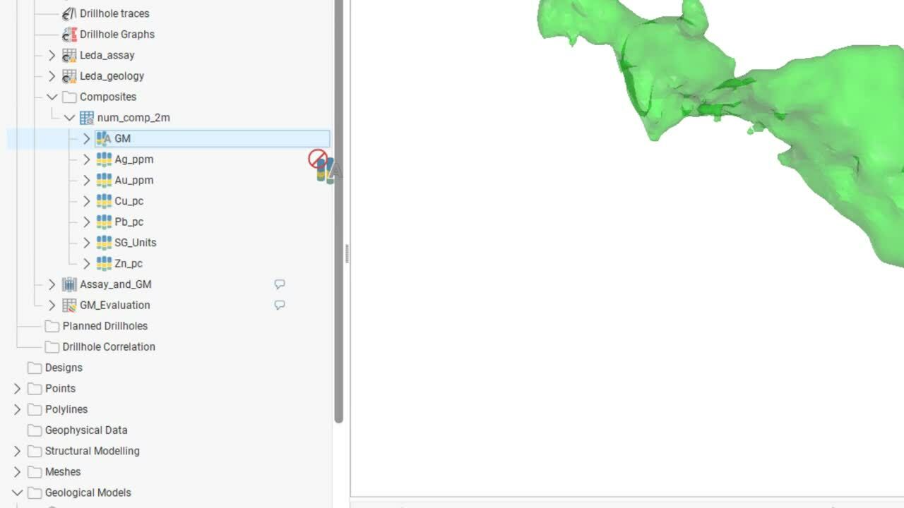
[00:09:57.930]And you’ll notice that the GM,

[00:10:00.960]the geological model evaluation is there as a column,

[00:10:06.620]where previously we would have had to do

[00:10:09.730]a separate merge table and combine the assays

[00:10:14.320]with the GM evaluation, so that’s processed.

[00:10:18.780]Let’s how the look at the GM, there it is.

[00:10:23.610]Flat traces we can make them rendered tubes,

[00:10:29.370]a three meter radius,

[00:10:31.800]and we can also look at our composited zinc here

[00:10:36.180]just to check.

[00:10:37.013]So those are all two meter composites.

[00:10:41.230]The next new feature I’d like to show you

[00:10:43.410]are drillhole calculations.

[00:10:45.350]I think this is an important one

[00:10:46.700]that you’re going to appreciate.

[00:10:48.210]So let’s say for instance we want to add a capped column

[00:10:52.000]to an assay table.

[00:10:54.750]So here we have our Leda assays.

[00:10:57.120]We can look at our silver,

[00:10:58.650]I believe there are some outliers in silver,

[00:11:01.210]and just have a look at the unit various statistics.

[00:11:03.770]So here’s a log probability plot of silver,

[00:11:07.100]and it does look like there could be a tail here

[00:11:09.770]at two, three, four, five,

[00:11:11.820]above 500 perhaps around 600 grams per ton.

[00:11:16.030]We can look at the histogram.

[00:11:18.520]And we can see that similarly there’s the tail there,

[00:11:21.360]so without further analysis, let’s choose 600 grams

[00:11:26.600]as a reasonable capping value.

[00:11:30.130]So then we go to our Leda assay table,

[00:11:33.300]right click and select calculations.

[00:11:36.690]And we get the same calculations and filters panel that

[00:11:41.010]was available for block modeling and for points

[00:11:44.470]in the most recent release.

[00:11:46.150]Now I’m going to add

[00:11:47.140]a new numeric calculation.

[00:11:51.270]Going to call it a Ag Cap,

[00:11:56.010]click okay and then write a short if statement,

[00:12:01.450]if my silver

[00:12:05.120]is greater than 600,

[00:12:11.360]then the result is capped at 600.

[00:12:16.000]Otherwise it will get the silver value,

[00:12:20.700]no errors I’ll click save.

[00:12:23.670]And as it is saved,

[00:12:27.500]it is computed and it’s there now

[00:12:30.813]under calculations.

[00:12:32.440]These are the imported columns and the Ag Cap

[00:12:35.980]is there as a calculated column.

[00:12:39.270]Let’s just remove our numeric comp

[00:12:43.930]and then bring in the capped silver.

[00:12:47.890]And there’s the cap silver and of course you can select

[00:12:52.200]any of the other columns in the table from the dropdown.

[00:12:55.260]So there is capped and uncapped,

[00:12:59.020]go back to the capped and let’s have a look

[00:13:01.560]at the unit various statistics on that capped value.

[00:13:06.140]So we’ll have a look at the histogram of the log

[00:13:09.380]and there we can see our maximum value capped at 600

[00:13:13.470]so there is a new calculated column.

[00:13:17.770]The next thing we’ll have a look at are some

[00:13:19.900]of the mesh issues that we were talking about earlier.

[00:13:23.400]So let’s just clear the scene

[00:13:26.310]and collapse the project tree

[00:13:29.170]so that we can find things better.

[00:13:30.800]And here’s the meshes,

[00:13:32.600]and here we have meshes with issues.

[00:13:36.950]So here is a mesh with

[00:13:39.783]just we can look at the border edges.

[00:13:43.450]So there are the border edges.

[00:13:46.450]And in this case, we’ll just get that mesh into the scene.

[00:13:49.500]Now we can see that mesh

[00:13:52.880]has a hole in it identified by the mesh edge

[00:13:57.770]and if we want to repair this in another software,

[00:14:01.710]the source software we can right click and export that

[00:14:05.900]as a polyline, so a Leapfrog polyline file

[00:14:08.970]or any of the other supported exchange formats.

[00:14:13.730]DXF for instance,

[00:14:17.810]I will just clear these.

[00:14:21.090]And we have another issue here.

[00:14:24.250]Here we have a fault zone

[00:14:28.660]and there are some mesh issues showing up here somewhere.

[00:14:34.630]Let’s just hide that overall

[00:14:36.360]So there are still some remaining problems

[00:14:41.270]and it’s showing us where

[00:14:44.685]we can now export these and send them back for repair.

[00:14:51.140]Let’s get rid of these and have a look

[00:14:54.160]at the fault zone mesh, there’s an issues here as well.

[00:14:59.160]There’s our fault so a mesh,

[00:15:02.190]and we have still some non-manifold edges

[00:15:07.090]that need to be addressed.

[00:15:08.980]And they’re just very, very small objects

[00:15:13.480]in that mesh.

[00:15:15.280]But now we can export those non manifold edges,

[00:15:21.630]again as any one of the supported file formats.

[00:15:25.990]And we could perhaps fix these in the source software

[00:15:31.780]where the mesh came from.

[00:15:35.898]The next new feature I’ll show you is the ability

[00:15:38.630]to lock the total sill in the variogram.

[00:15:41.360]So let’s remove our meshes which is collapsed meshes,

[00:15:46.340]go down to the estimation folder

[00:15:49.270]and let’s have a look at zinc in the domain MLS1.

[00:15:54.280]Spatial models is where our variograms are,

[00:15:56.740]we have some already built here as the variogram model

[00:16:01.280]for zinc in LMS1.

[00:16:05.330]The opening page always shows us

[00:16:07.017]the three nested variograms.

[00:16:09.900]And if we look at the radial plot,

[00:16:12.240]we can see the orientation

[00:16:14.480]of our experimental models

[00:16:18.300]and experiment variogram and models.

[00:16:21.060]And let’s go now to the major access tab.

[00:16:24.510]This one has already been reasonably modeled

[00:16:28.850]or modeled reasonably well.

[00:16:32.320]And what I’ll show you is that here is the lock

[00:16:35.150]that we can use that will enable

[00:16:38.460]the total sill to remain fixed.

[00:16:41.170]So currently I can move my sill around

[00:16:44.740]and it is free as I changed the range,

[00:16:49.360]perhaps I could inadvertently alter my model.

[00:16:53.520]So I think I’ll just go back to set this

[00:16:58.630]to be 0.3, the second structure 0.3,

[00:17:01.960]so that my three models now sum to one.

[00:17:06.240]I want to put that handle back into its position here

[00:17:12.090]out to the maximum range there.

[00:17:13.940]So I’m going to click on the lock.

[00:17:16.560]And now when I drag that handle,

[00:17:19.870]it is not changing the gamma values.

[00:17:24.070]I can just put it into position

[00:17:26.370]and let’s just make that to be 160 meters full stop.

[00:17:32.590]This is a good opportunity to show you as well

[00:17:37.145]the four new model types that we’ve added.

[00:17:40.180]Perhaps we can close this one and add a new variogram

[00:17:43.840]I’ll just discard any changes that we made there,

[00:17:48.090]and go down to our spatial models

[00:17:50.380]and select new variogram model.

[00:17:56.430]And go to the access aligned variograms let’s set.

[00:18:02.840]Well, we need to put in a reasonable Dip

[00:18:05.370]for our LMS1

[00:18:09.780]Dip Azimuth.

[00:18:11.700]I can remember these values pretty well.

[00:18:19.975]We’ll just look at the one structure

[00:18:21.700]or a model with one structure so we can see what

[00:18:25.440]the shape of these curves looked like

[00:18:27.000]when we changed the different model types.

[00:18:30.930]So we have our spherical model

[00:18:34.920]and spheroidals, you’ll recognize those.

[00:18:38.550]And you’ll see that a portion of the model is linear

[00:18:43.060]before it starts to rise to the sill.

[00:18:46.490]And if we look at the exponential

[00:18:48.710]now it is steeper near the origin.

[00:18:50.830]There really isn’t a linear portion of the curve any longer.

[00:18:55.270]This does suit metals quite well

[00:18:58.790]like silver, gold, even the zinc.

[00:19:02.530]If we look at our lag distance here,

[00:19:05.640]I’ll just increase it to be 15.

[00:19:09.510]We can see now that the curve

[00:19:11.780]is approaching the sill,

[00:19:15.490]I can move that.

[00:19:19.720]Let’s just lock the sill.

[00:19:25.100]It looks like I’ll need another structure to model that,

[00:19:27.410]but I’m capturing the close range continuity

[00:19:31.680]a little bit better.

[00:19:33.730]Now, some of the other models here is the Gaussian,

[00:19:37.280]you’ll see that it is showing

[00:19:39.860]much better continuity near the origin,

[00:19:43.900]similarly cubic, slightly different shapes

[00:19:47.910]in the generalized Cauchy.

[00:19:50.351]With these models of course,

[00:19:52.850]if you’re estimating metals,

[00:19:54.400]you may find that it creates a bit of a smoothing

[00:19:58.490]near the blocks.

[00:20:01.580]This is introduced really

[00:20:04.270]for contaminants and things like that.

[00:20:07.070]So I think we can close this and I’ll just discard

[00:20:11.010]those changes again.

[00:20:16.340]The next feature to show you

[00:20:17.570]is the index filter refinement.

[00:20:21.350]So let’s just collapse the tree again

[00:20:23.000]and go to our block model.

[00:20:25.890]Here’s the block model.

[00:20:28.150]And I have a sub block model that I am more familiar with.

[00:20:32.575]And just have a look at the zinc model here

[00:20:37.060]in one of our domains.

[00:20:38.720]So we have kriged zinc in LMS1,

[00:20:42.140]that’s what I’m looking for.

[00:20:44.620]It’ll take a moment to come into the scene,

[00:20:46.290]so there we have it.

[00:20:49.920]And now for visualization we will look at the indexes.

[00:20:55.730]So if we select a subset,

[00:20:59.570]and then right click on the X, I’ll all of my values in X.

[00:21:05.870]I’m going to click on the Y,

[00:21:08.600]but I’m going to make that to just one column

[00:21:13.440]and a right click will give you the full range,

[00:21:16.670]a double click will bring the range

[00:21:22.107]to just into just into the center,

[00:21:24.110]makes it a little bit easier to refine.

[00:21:27.820]And so there is a quick little subset of blocks.

[00:21:32.610]If we change to a slice,

[00:21:35.370]and now I’ll will first off right click to expand

[00:21:38.570]that to the full range,

[00:21:40.560]and bring it right back on the Y and Z directions.

[00:21:45.190]And now I can see where my model is

[00:21:50.000]as a slice.

[00:21:50.920]And I’ll just bring that into one column

[00:21:54.610]in my block model.

[00:21:58.740]So that does make it a little bit easier

[00:22:00.350]to see what’s going on.

[00:22:02.653]I’ll just remove that filter

[00:22:06.350]and let’s have a look at what this looks like

[00:22:09.820]in a swath plot sorry.

[00:22:12.360]Double click on the swath plot to open it.

[00:22:15.930]And now I can see this is an X,

[00:22:18.920]and if I right click,

[00:22:20.490]I can see the full range through the block model

[00:22:23.930]and of course this region here is where that other lens,

[00:22:27.540]the LMS2 lens is setting.

[00:22:29.530]So we want to just double click on our index filter

[00:22:34.150]and it zooms in, the bracket is a reasonable bracket

[00:22:39.120]and I can then just adjust it so that I’m not seeing

[00:22:42.960]that huge white area of empty space

[00:22:46.460]there in my swath plot.

[00:22:49.200]The last thing I’d like to show you and definitely not least

[00:22:51.960]is the estimation parameter report.

[00:22:54.880]So let’s go to our estimations folder.

[00:22:57.740]Right Click and select parameter report.

[00:23:01.970]This is an important new addition.

[00:23:04.040]So it opens to the domain estimation tab,

[00:23:06.320]we can see the different domain estimations that we have.

[00:23:11.270]There’s also the interpolant tab

[00:23:15.310]showing us the different interpolants, the search tab,

[00:23:19.630]outputs and variograms.

[00:23:23.566]And of course, these are all filterable.

[00:23:25.460]If we go to our domain filter,

[00:23:27.450]we can select all, none,

[00:23:29.550]or just select off of the list.

[00:23:33.280]On the value filter, we only had silver and lead there

[00:23:36.850]and let’s add SG and zinc.

[00:23:40.100]Now these filters are just for visualization.

[00:23:43.020]If we do export this,

[00:23:47.065]it’s the full grid everything is there.

[00:23:49.540]So now in our interpolant tab,

[00:23:51.900]I want to try the search tab.

[00:23:53.700]We can sort these columns.

[00:24:00.890]Sorting will give us a quick idea of

[00:24:06.920]if there are any values that are out of range perhaps that

[00:24:10.100]we need to adjust.

[00:24:12.890]And let’s see on the interpolant tab now,

[00:24:17.020]these will also give us a link to

[00:24:19.340]the tab in our interpolant as well.

[00:24:23.500]So let’s double click on our kriged zinc in LMS1,

[00:24:28.490]and it takes us right to the interpolant tab.

[00:24:32.620]Likewise, if I want to see a variogram,

[00:24:35.482]I’ll just double click on the variogram

[00:24:38.760]and it will take me directly there.

[00:24:42.440]So a very nice link,

[00:24:47.140]adding a little bit of efficiency to our estimations,

[00:24:50.810]and of course, everything in one place.

[00:24:52.850]And we can export this now to a parameters file.

[00:24:57.610]So we’ll click on save.

[00:25:00.290]Let’s have a look at what this is in Excel.

[00:25:04.890]Where’s my parameters?

[00:25:05.970]It’s parameters.

[00:25:09.840]So the same tabs, domain estimation,

[00:25:11.920]interpolant, search, outputs, and variogram.

[00:25:15.140]And everything is all there

[00:25:20.150]so that we can communicate and collaborate.

[00:25:22.920]And we have a record of what we’ve done

[00:25:26.030]when we need to show our reviewers.

[00:25:32.870]That brings us to the end of the demo.

[00:25:36.220]So that is the end of our new product release

[00:25:39.450]for Edge version 4.0.1.

[00:25:42.150]And I thank you for watching,

[00:25:44.200]goodbye till next time.

[00:00:01.600]<v Instructor>Welcome to the release webinar</v>

[00:00:03.380]for Leapfrog Geo version 6.0.1

[00:00:06.700]and Edge Extension version 4.0.1.

[00:00:11.210]Please note, we have released these updated versions

[00:00:14.500]as we identified an issue which may have prevented you

[00:00:17.490]from accessing the new version of the software.

[00:00:20.760]We want to deliver a great user experience

[00:00:23.430]and are pleased to say, this is now fixed,

[00:00:26.190]and the new release is ready for you to download.

[00:00:30.130]This new release is a big one for Seequent,

[00:00:32.730]Leapfrog not only looks different,

[00:00:34.900]but has some key features that many customers

[00:00:37.130]have been asking for.

[00:00:39.180]But before we get going,

[00:00:40.590]there are a couple of go-to meeting logistics.

[00:00:43.690]If you take a look at the go-to webinar dialogue panel,

[00:00:46.800]you should see a place for questions.

[00:00:49.080]Can you take a moment to type yes if you can hear me?

[00:00:53.430]I won’t be answering questions during the webinar,

[00:00:56.020]so please use this panel to enter your questions

[00:00:59.060]and I will answer them with a personal email

[00:01:01.750]after the webinar ends.

[00:01:04.700]Here is an overview of the main themes we will be discussing

[00:01:07.510]in this product update.

[00:01:09.540]I will introduce some of them here,

[00:01:11.610]and describe them in more detail later in the webinar.

[00:01:15.390]We have a new user interface,

[00:01:18.940]improvements to drillholes,

[00:01:21.700]better mesh handling, estimation parameter management,

[00:01:26.890]block model reporting improvements, and more.

[00:01:31.910]The you Leapfrog user interface is the first thing

[00:01:34.390]we want to talk about because there is no escaping

[00:01:37.120]the fact that it looks different to the last release.

[00:01:40.920]Seequent has put a huge amount of effort into updating

[00:01:43.800]the building blocks of Leapfrog, and this has enabled us

[00:01:46.940]to introduce a new user experience.

[00:01:51.160]The new user interface of Leapfrog is sleek, streamlined,

[00:01:55.490]and brings cohesion

[00:01:56.560]across the Seequent portfolio of products.

[00:01:59.920]While it may appear quite different at first glance,

[00:02:02.770]all of the functionality remains in exactly the same place

[00:02:06.290]as it was before.

[00:02:08.890]Secondly, we wanted to show you the effort we have put

[00:02:11.680]into making your Leapfrog experience better

[00:02:14.240]when using some of the main functionality.

[00:02:17.000]We have made improvements to the drillhole database

[00:02:19.740]so that your modeling is based on quick to load, accurate

[00:02:23.260]and easy to update data.

[00:02:26.740]We’ve made improvements to the processing of tasks

[00:02:29.360]in parallel so that your drilling data can process

[00:02:33.300]and reload substantially quicker for some projects.

[00:02:36.610]In some instances, we have reduced the processing time

[00:02:40.090]by over 40%.

[00:02:43.150]To make importing drilling data easier,

[00:02:45.470]you can now import your downhole points

[00:02:47.640]from structural data for instance,

[00:02:49.870]at the same time as your collar, survey,

[00:02:52.150]and interval tables.

[00:02:54.860]Made a mistake when importing,

[00:02:56.590]or no longer require one of your data columns?

[00:02:59.730]Leapfrog will now allow you to rename

[00:03:02.280]and delete your imported columns.

[00:03:04.810]This will enable you to keep your data

[00:03:06.800]up to date and relevant.

[00:03:09.530]This option is available for all data tables,

[00:03:12.250]including collars, interval tables, GIS,

[00:03:15.800]and structural data.

[00:03:18.510]And now what we think is the most exciting addition

[00:03:20.850]to the drillholes, calculations.

[00:03:24.140]Use this tab to write calculations

[00:03:26.160]that will categorize, combine or reclassify your data.

[00:03:30.730]You can for instance, add a new calculated column

[00:03:33.460]for capped assay values prior to compositing.

[00:03:37.460]Calculations are also available for calculated points

[00:03:41.000]such as mid points, guide points and grade of points.

[00:03:46.090]Dealing with invalid measures can be problematic,

[00:03:49.080]it is often hard to locate

[00:03:50.470]where the problems are to fix them,

[00:03:52.320]we have made some changes in this release

[00:03:54.200]to make this easier.

[00:03:56.550]Firstly, we have improved the way we categorize

[00:03:59.540]the mesh issues.

[00:04:01.100]It is now clear which errors the mesh contains

[00:04:03.840]from the tree view directly,

[00:04:06.000]instead of having to look at the properties of the mesh.

[00:04:10.000]Secondly, the tickbox to view the border edge on a mesh

[00:04:13.540]has now been turned into its own separate object.

[00:04:16.870]This means you can view the location

[00:04:19.830]of the issue in the scene independent of the mesh.

[00:04:23.460]In addition, the border edges object can be exported

[00:04:26.860]as a polyline file, which can be visualized

[00:04:29.950]in the source software of the mesh.

[00:04:33.110]We have also added another categorization to the way

[00:04:36.270]we define non-manifold meshes,

[00:04:39.560]as well as being able to view the non=manifold edges

[00:04:42.300]in the scene as their own object.

[00:04:44.440]We have also enabled some non manifold meshes to be used

[00:04:47.860]that were once unusable.

[00:04:50.750]Non-manifold meshes with an even number

[00:04:53.100]of adjoining triangles are now usable.

[00:04:56.240]However, non manifold meshes with an odd number

[00:04:59.140]of adjoining triangles will result

[00:05:01.170]in an object named odd non-manifold edges,

[00:05:04.860]and these will remain unusable.

[00:05:08.030]For more information on the improvements in Geo,

[00:05:10.520]please watch the Leapfrog Geo version 6.0.1 release webinar

[00:05:14.580]and video.

[00:05:16.810]And now a highly requested new feature for block estimation.

[00:05:21.320]Leapfrog has developed the estimation parameter report

[00:05:25.000]to help make multi-domain estimation more efficient.

[00:05:30.020]This is the first step in an initiative to describe,

[00:05:33.590]to transform the creation and management

[00:05:35.740]of resource estimation parameters in Edge.

[00:05:39.510]The parameter report allows you to view

[00:05:41.760]the estimation parameters for every estimator

[00:05:44.410]in your project.

[00:05:46.600]Use the domain and filters to refine your parameter view.

[00:05:50.920]Swap between tabs to change your parameters.

[00:05:54.340]Click in the sill to open the relevant object for editing.

[00:05:57.960]Click on the headers to sort the rows

[00:05:59.670]to identify patterns or errors.

[00:06:02.270]Use the export button to export your parameters

[00:06:05.030]to an Excel spreadsheet.

[00:06:06.770]Regardless of your filtering, the entire parameter report

[00:06:10.080]will export to allow for filtering in Excel.

[00:06:13.670]Tabs and the parameter report will be displayed

[00:06:16.280]in different worksheets in Excel.

[00:06:19.280]In this release, we have tried to identify some improvements

[00:06:22.120]that will make your estimation easier.

[00:06:25.320]We have made improvements to the variogram tab

[00:06:28.050]to help you with your variography.

[00:06:30.690]Firstly based on feedback,

[00:06:33.000]we have added the option to lock the total sill,

[00:06:36.670]click on the padlock to lock the total sill.

[00:06:39.370]Changes made to the structures will no longer affect

[00:06:42.030]the total sill, this is especially useful

[00:06:45.120]for fitting variograms with two structures.

[00:06:48.360]We have also added four more variogram model types

[00:06:51.730]to provide additional flexibility when modeling variables,

[00:06:55.380]which have high continuity and high local correlation.

[00:06:59.900]The exponential model, which is steeper at the origin

[00:07:02.580]than the spherical or spheroidal model

[00:07:04.750]and is commonly used for metals.

[00:07:07.090]Gaussian, cubic, and generalized Cauchy,

[00:07:09.990]which are more continuous near the origin.

[00:07:13.670]Here are some usability improvements that we think will help

[00:07:16.280]you when creating your estimation project.

[00:07:19.960]When creating a numeric composite within a subset of codes,

[00:07:23.370]we have now added the resulting lithology column

[00:07:25.820]from the base column used.

[00:07:28.270]This means that your numeric composite table

[00:07:30.880]is already merged with the base column,

[00:07:33.560]reducing the need to make merge tables,

[00:07:36.090]to combine your numeric composite

[00:07:37.910]with your lithology domain.

[00:07:40.280]With large block models it can be difficult to use

[00:07:43.150]the index filter to capture the blocks

[00:07:45.090]you want to visualize.

[00:07:46.820]We have added an extra control to allow you to zoom

[00:07:49.980]into the filter range and refine it further.

[00:07:53.140]This feature is used in block visualization

[00:07:55.840]and in swath plots.

[00:07:58.280]Lastly, we have made some improvements

[00:08:00.070]to block model reporting to make it more flexible

[00:08:03.300]for different types of resources.

[00:08:05.820]The ability to report below the cutoff is helpful

[00:08:09.700]for those reporting on industrial minerals or contaminants.

[00:08:13.710]We have added carats as a reporting unit for those looking

[00:08:16.630]to estimate diamond resources.

[00:08:19.190]And for those looking to create a great tonnage report,

[00:08:22.570]we have also added the ability to report below the cutoff.

[00:08:26.610]This will invert the grade tonnage curve.

[00:08:30.040]I will now demonstrate some of the new features

[00:08:32.100]in Leapfrog Edge version 4.0.1.

[00:08:36.560]The first new feature I’d like to show you

[00:08:38.710]is the improvement in numeric compositing.

[00:08:42.570]So we have the Leda training project here.

[00:08:45.650]Those of you who have taken training from us

[00:08:48.040]will recognize it immediately.

[00:08:50.010]Now I’m going to right click on composites,

[00:08:53.100]select a new numeric composite

[00:08:55.980]using a subset of codes ’cause I want to see the lithology.

[00:09:00.500]The base column will come

[00:09:01.680]from the geological model evaluated

[00:09:04.710]onto the drillhole traces.

[00:09:07.410]And we’ll select a logical compositing length,

[00:09:12.620]two meters in this case, with a minimum coverage

[00:09:15.340]of 0% so that every interval has a chance

[00:09:19.030]of becoming a valid composite.

[00:09:21.470]And for short length composites,

[00:09:25.320]if there’s a residual length less than a meter,

[00:09:27.860]we will distribute it equally amongst

[00:09:31.296]all of the composites in the interval.

[00:09:34.450]And we’ll just give this a nice name call it the numb comp,

[00:09:39.360]I like to shorten it a little bit, two meters.

[00:09:43.410]And the output columns we will grab

[00:09:46.130]all of our Leda assay columns,

[00:09:50.700]and then click okay.

[00:09:53.770]So we’ll see that the structure of the table

[00:09:56.290]is already there.

[00:09:57.930]And you’ll notice that the GM,

[00:10:00.960]the geological model evaluation is there as a column,

[00:10:06.620]where previously we would have had to do

[00:10:09.730]a separate merge table and combine the assays

[00:10:14.320]with the GM evaluation, so that’s processed.

[00:10:18.780]Let’s how the look at the GM, there it is.

[00:10:23.610]Flat traces we can make them rendered tubes,

[00:10:29.370]a three meter radius,

[00:10:31.800]and we can also look at our composited zinc here

[00:10:36.180]just to check.

[00:10:37.013]So those are all two meter composites.

[00:10:41.230]The next new feature I’d like to show you

[00:10:43.410]are drillhole calculations.

[00:10:45.350]I think this is an important one

[00:10:46.700]that you’re going to appreciate.

[00:10:48.210]So let’s say for instance we want to add a capped column

[00:10:52.000]to an assay table.

[00:10:54.750]So here we have our Leda assays.

[00:10:57.120]We can look at our silver,

[00:10:58.650]I believe there are some outliers in silver,

[00:11:01.210]and just have a look at the unit various statistics.

[00:11:03.770]So here’s a log probability plot of silver,

[00:11:07.100]and it does look like there could be a tail here

[00:11:09.770]at two, three, four, five,

[00:11:11.820]above 500 perhaps around 600 grams per ton.

[00:11:16.030]We can look at the histogram.

[00:11:18.520]And we can see that similarly there’s the tail there,

[00:11:21.360]so without further analysis, let’s choose 600 grams

[00:11:26.600]as a reasonable capping value.

[00:11:30.130]So then we go to our Leda assay table,

[00:11:33.300]right click and select calculations.

[00:11:36.690]And we get the same calculations and filters panel that

[00:11:41.010]was available for block modeling and for points

[00:11:44.470]in the most recent release.

[00:11:46.150]Now I’m going to add

[00:11:47.140]a new numeric calculation.

[00:11:51.270]Going to call it a Ag Cap,

[00:11:56.010]click okay and then write a short if statement,

[00:12:01.450]if my silver

[00:12:05.120]is greater than 600,

[00:12:11.360]then the result is capped at 600.

[00:12:16.000]Otherwise it will get the silver value,

[00:12:20.700]no errors I’ll click save.

[00:12:23.670]And as it is saved,

[00:12:27.500]it is computed and it’s there now

[00:12:30.813]under calculations.

[00:12:32.440]These are the imported columns and the Ag Cap

[00:12:35.980]is there as a calculated column.

[00:12:39.270]Let’s just remove our numeric comp

[00:12:43.930]and then bring in the capped silver.

[00:12:47.890]And there’s the cap silver and of course you can select

[00:12:52.200]any of the other columns in the table from the dropdown.

[00:12:55.260]So there is capped and uncapped,

[00:12:59.020]go back to the capped and let’s have a look

[00:13:01.560]at the unit various statistics on that capped value.

[00:13:06.140]So we’ll have a look at the histogram of the log

[00:13:09.380]and there we can see our maximum value capped at 600

[00:13:13.470]so there is a new calculated column.

[00:13:17.770]The next thing we’ll have a look at are some

[00:13:19.900]of the mesh issues that we were talking about earlier.

[00:13:23.400]So let’s just clear the scene

[00:13:26.310]and collapse the project tree

[00:13:29.170]so that we can find things better.

[00:13:30.800]And here’s the meshes,

[00:13:32.600]and here we have meshes with issues.

[00:13:36.950]So here is a mesh with

[00:13:39.783]just we can look at the border edges.

[00:13:43.450]So there are the border edges.

[00:13:46.450]And in this case, we’ll just get that mesh into the scene.

[00:13:49.500]Now we can see that mesh

[00:13:52.880]has a hole in it identified by the mesh edge

[00:13:57.770]and if we want to repair this in another software,

[00:14:01.710]the source software we can right click and export that

[00:14:05.900]as a polyline, so a Leapfrog polyline file

[00:14:08.970]or any of the other supported exchange formats.

[00:14:13.730]DXF for instance,

[00:14:17.810]I will just clear these.

[00:14:21.090]And we have another issue here.

[00:14:24.250]Here we have a fault zone

[00:14:28.660]and there are some mesh issues showing up here somewhere.

[00:14:34.630]Let’s just hide that overall

[00:14:36.360]So there are still some remaining problems

[00:14:41.270]and it’s showing us where

[00:14:44.685]we can now export these and send them back for repair.

[00:14:51.140]Let’s get rid of these and have a look

[00:14:54.160]at the fault zone mesh, there’s an issues here as well.

[00:14:59.160]There’s our fault so a mesh,

[00:15:02.190]and we have still some non-manifold edges

[00:15:07.090]that need to be addressed.

[00:15:08.980]And they’re just very, very small objects

[00:15:13.480]in that mesh.

[00:15:15.280]But now we can export those non manifold edges,

[00:15:21.630]again as any one of the supported file formats.

[00:15:25.990]And we could perhaps fix these in the source software

[00:15:31.780]where the mesh came from.

[00:15:35.898]The next new feature I’ll show you is the ability

[00:15:38.630]to lock the total sill in the variogram.

[00:15:41.360]So let’s remove our meshes which is collapsed meshes,

[00:15:46.340]go down to the estimation folder

[00:15:49.270]and let’s have a look at zinc in the domain MLS1.

[00:15:54.280]Spatial models is where our variograms are,

[00:15:56.740]we have some already built here as the variogram model

[00:16:01.280]for zinc in LMS1.

[00:16:05.330]The opening page always shows us

[00:16:07.017]the three nested variograms.

[00:16:09.900]And if we look at the radial plot,

[00:16:12.240]we can see the orientation

[00:16:14.480]of our experimental models

[00:16:18.300]and experiment variogram and models.

[00:16:21.060]And let’s go now to the major access tab.

[00:16:24.510]This one has already been reasonably modeled

[00:16:28.850]or modeled reasonably well.

[00:16:32.320]And what I’ll show you is that here is the lock

[00:16:35.150]that we can use that will enable

[00:16:38.460]the total sill to remain fixed.

[00:16:41.170]So currently I can move my sill around

[00:16:44.740]and it is free as I changed the range,

[00:16:49.360]perhaps I could inadvertently alter my model.

[00:16:53.520]So I think I’ll just go back to set this

[00:16:58.630]to be 0.3, the second structure 0.3,

[00:17:01.960]so that my three models now sum to one.

[00:17:06.240]I want to put that handle back into its position here

[00:17:12.090]out to the maximum range there.

[00:17:13.940]So I’m going to click on the lock.

[00:17:16.560]And now when I drag that handle,

[00:17:19.870]it is not changing the gamma values.

[00:17:24.070]I can just put it into position

[00:17:26.370]and let’s just make that to be 160 meters full stop.

[00:17:32.590]This is a good opportunity to show you as well

[00:17:37.145]the four new model types that we’ve added.

[00:17:40.180]Perhaps we can close this one and add a new variogram

[00:17:43.840]I’ll just discard any changes that we made there,

[00:17:48.090]and go down to our spatial models

[00:17:50.380]and select new variogram model.

[00:17:56.430]And go to the access aligned variograms let’s set.

[00:18:02.840]Well, we need to put in a reasonable Dip

[00:18:05.370]for our LMS1

[00:18:09.780]Dip Azimuth.

[00:18:11.700]I can remember these values pretty well.

[00:18:19.975]We’ll just look at the one structure

[00:18:21.700]or a model with one structure so we can see what

[00:18:25.440]the shape of these curves looked like

[00:18:27.000]when we changed the different model types.

[00:18:30.930]So we have our spherical model

[00:18:34.920]and spheroidals, you’ll recognize those.

[00:18:38.550]And you’ll see that a portion of the model is linear

[00:18:43.060]before it starts to rise to the sill.

[00:18:46.490]And if we look at the exponential

[00:18:48.710]now it is steeper near the origin.

[00:18:50.830]There really isn’t a linear portion of the curve any longer.

[00:18:55.270]This does suit metals quite well

[00:18:58.790]like silver, gold, even the zinc.

[00:19:02.530]If we look at our lag distance here,

[00:19:05.640]I’ll just increase it to be 15.

[00:19:09.510]We can see now that the curve

[00:19:11.780]is approaching the sill,

[00:19:15.490]I can move that.

[00:19:19.720]Let’s just lock the sill.

[00:19:25.100]It looks like I’ll need another structure to model that,

[00:19:27.410]but I’m capturing the close range continuity

[00:19:31.680]a little bit better.

[00:19:33.730]Now, some of the other models here is the Gaussian,

[00:19:37.280]you’ll see that it is showing

[00:19:39.860]much better continuity near the origin,

[00:19:43.900]similarly cubic, slightly different shapes

[00:19:47.910]in the generalized Cauchy.

[00:19:50.351]With these models of course,

[00:19:52.850]if you’re estimating metals,

[00:19:54.400]you may find that it creates a bit of a smoothing

[00:19:58.490]near the blocks.

[00:20:01.580]This is introduced really

[00:20:04.270]for contaminants and things like that.

[00:20:07.070]So I think we can close this and I’ll just discard

[00:20:11.010]those changes again.

[00:20:16.340]The next feature to show you

[00:20:17.570]is the index filter refinement.

[00:20:21.350]So let’s just collapse the tree again

[00:20:23.000]and go to our block model.

[00:20:25.890]Here’s the block model.

[00:20:28.150]And I have a sub block model that I am more familiar with.

[00:20:32.575]And just have a look at the zinc model here

[00:20:37.060]in one of our domains.

[00:20:38.720]So we have kriged zinc in LMS1,

[00:20:42.140]that’s what I’m looking for.

[00:20:44.620]It’ll take a moment to come into the scene,

[00:20:46.290]so there we have it.

[00:20:49.920]And now for visualization we will look at the indexes.

[00:20:55.730]So if we select a subset,

[00:20:59.570]and then right click on the X, I’ll all of my values in X.

[00:21:05.870]I’m going to click on the Y,

[00:21:08.600]but I’m going to make that to just one column

[00:21:13.440]and a right click will give you the full range,

[00:21:16.670]a double click will bring the range

[00:21:22.107]to just into just into the center,

[00:21:24.110]makes it a little bit easier to refine.

[00:21:27.820]And so there is a quick little subset of blocks.

[00:21:32.610]If we change to a slice,

[00:21:35.370]and now I’ll will first off right click to expand

[00:21:38.570]that to the full range,

[00:21:40.560]and bring it right back on the Y and Z directions.

[00:21:45.190]And now I can see where my model is

[00:21:50.000]as a slice.

[00:21:50.920]And I’ll just bring that into one column

[00:21:54.610]in my block model.

[00:21:58.740]So that does make it a little bit easier

[00:22:00.350]to see what’s going on.

[00:22:02.653]I’ll just remove that filter

[00:22:06.350]and let’s have a look at what this looks like

[00:22:09.820]in a swath plot sorry.

[00:22:12.360]Double click on the swath plot to open it.

[00:22:15.930]And now I can see this is an X,

[00:22:18.920]and if I right click,

[00:22:20.490]I can see the full range through the block model

[00:22:23.930]and of course this region here is where that other lens,

[00:22:27.540]the LMS2 lens is setting.

[00:22:29.530]So we want to just double click on our index filter

[00:22:34.150]and it zooms in, the bracket is a reasonable bracket

[00:22:39.120]and I can then just adjust it so that I’m not seeing

[00:22:42.960]that huge white area of empty space

[00:22:46.460]there in my swath plot.

[00:22:49.200]The last thing I’d like to show you and definitely not least

[00:22:51.960]is the estimation parameter report.

[00:22:54.880]So let’s go to our estimations folder.

[00:22:57.740]Right Click and select parameter report.

[00:23:01.970]This is an important new addition.

[00:23:04.040]So it opens to the domain estimation tab,

[00:23:06.320]we can see the different domain estimations that we have.

[00:23:11.270]There’s also the interpolant tab

[00:23:15.310]showing us the different interpolants, the search tab,

[00:23:19.630]outputs and variograms.

[00:23:23.566]And of course, these are all filterable.

[00:23:25.460]If we go to our domain filter,

[00:23:27.450]we can select all, none,

[00:23:29.550]or just select off of the list.

[00:23:33.280]On the value filter, we only had silver and lead there

[00:23:36.850]and let’s add SG and zinc.

[00:23:40.100]Now these filters are just for visualization.

[00:23:43.020]If we do export this,

[00:23:47.065]it’s the full grid everything is there.

[00:23:49.540]So now in our interpolant tab,

[00:23:51.900]I want to try the search tab.

[00:23:53.700]We can sort these columns.

[00:24:00.890]Sorting will give us a quick idea of

[00:24:06.920]if there are any values that are out of range perhaps that

[00:24:10.100]we need to adjust.

[00:24:12.890]And let’s see on the interpolant tab now,

[00:24:17.020]these will also give us a link to

[00:24:19.340]the tab in our interpolant as well.

[00:24:23.500]So let’s double click on our kriged zinc in LMS1,

[00:24:28.490]and it takes us right to the interpolant tab.

[00:24:32.620]Likewise, if I want to see a variogram,

[00:24:35.482]I’ll just double click on the variogram

[00:24:38.760]and it will take me directly there.

[00:24:42.440]So a very nice link,

[00:24:47.140]adding a little bit of efficiency to our estimations,

[00:24:50.810]and of course, everything in one place.

[00:24:52.850]And we can export this now to a parameters file.

[00:24:57.610]So we’ll click on save.

[00:25:00.290]Let’s have a look at what this is in Excel.

[00:25:04.890]Where’s my parameters?

[00:25:05.970]It’s parameters.

[00:25:09.840]So the same tabs, domain estimation,

[00:25:11.920]interpolant, search, outputs, and variogram.

[00:25:15.140]And everything is all there

[00:25:20.150]so that we can communicate and collaborate.

[00:25:22.920]And we have a record of what we’ve done

[00:25:26.030]when we need to show our reviewers.

[00:25:32.870]That brings us to the end of the demo.

[00:25:36.220]So that is the end of our new product release

[00:25:39.450]for Edge version 4.0.1.

[00:25:42.150]And I thank you for watching,

[00:25:44.200]goodbye till next time.