Introduction to Leapfrog Edge, a dynamic grade thickness workflow (Remote Roundup 2021)

Overview

Video Transcript

[00:00:00.899]
(gentle music)

[00:00:10.870]
<v Peter>Good morning or good afternoon everyone</v>

[00:00:14.078]
from wherever you’re attending.

[00:00:14.911]
I’m a professional geologist

[00:00:17.462]
with a few decades of experience

[00:00:18.470]
in mineral exploration and mining.

[00:00:20.160]
And I’ve focused mainly on long-term

[00:00:23.760]
mineral resource estimates in a variety of commodities,

[00:00:27.810]
diamonds, base metals, copper, nickel, precious metals

[00:00:32.540]
and PGEs and through a variety of deposit styles

[00:00:36.950]
in North and South America and Asia.

[00:00:40.260]
The bulk of my experience

[00:00:41.920]
was spent at the Ekati Diamond Mine,

[00:00:44.490]
where I contributed to a team that did the resource updates

[00:00:48.476]
on 10-kimberlite pipes up there at the time.

[00:00:52.610]
And I was with Wood, formerly Amec Foster Wheeler

[00:00:56.610]
for nine years in the Mining $ Metals Consulting group.

[00:01:00.900]
I’ve been at Seequent now since October, 2018,

[00:01:03.360]
so just over two years

[00:01:06.512]
and I am on the technical team

[00:01:10.112]
supporting business development training

[00:01:12.699]
and providing technical support.

[00:01:13.790]
And I think a few of you

[00:01:15.886]
will probably have communicated with me in that respect.

[00:01:19.870]
And I do focus on the Leapfrog Edge

[00:01:24.150]
resource estimation tool in Geo.

[00:01:28.780]
So we’re going to cover

[00:01:31.870]
basically the estimation workflow in Edge.

[00:01:35.170]
So we’ll start with exploratory data analysis

[00:01:37.650]
and compositing, we’ll define a few estimators.

[00:01:41.330]
We’ll create a rotated sub-blocked block model.

[00:01:43.947]
And this is kind of the trick for doing

[00:01:45.940]
the grade-thickness calculation in Edge.

[00:01:48.960]
We’ll evaluate the estimators, validate the results.

[00:01:52.260]
Not thoroughly, but we will do a couple of checks

[00:01:55.449]
and then we’ll compose and evaluate

[00:01:56.810]
our grade-thickness calculations

[00:01:59.020]
and review the results.

[00:02:00.670]
And then of course,

[00:02:02.240]
our work is intended for another audience

[00:02:05.350]
and I’m picturing that the rotated

[00:02:08.523]
grade-thickness model will go to

[00:02:12.060]
engineers who will re-block it

[00:02:14.160]
and use it for their mine planning.

[00:02:16.920]
So I’m just going to stop my camera for now

[00:02:21.012]
so that, there we go, turning it off and we’ll carry on.

[00:02:25.290]
Now, this grade-thickness in Edge is one way to do it.

[00:02:29.820]
We also have presented in the past,

[00:02:33.076]
most recently at the Lyceum 2020 Tips &amp; Tricks

[00:02:37.500]
with Sarah Connolly presenting

[00:02:40.312]
and we’ll provide a link for you to this recording

[00:02:44.240]
that was done last fall.

[00:02:45.990]
So this is a way to do grade-thickness contouring in Geo,

[00:02:49.260]
if you don’t have Edge.

[00:02:53.280]
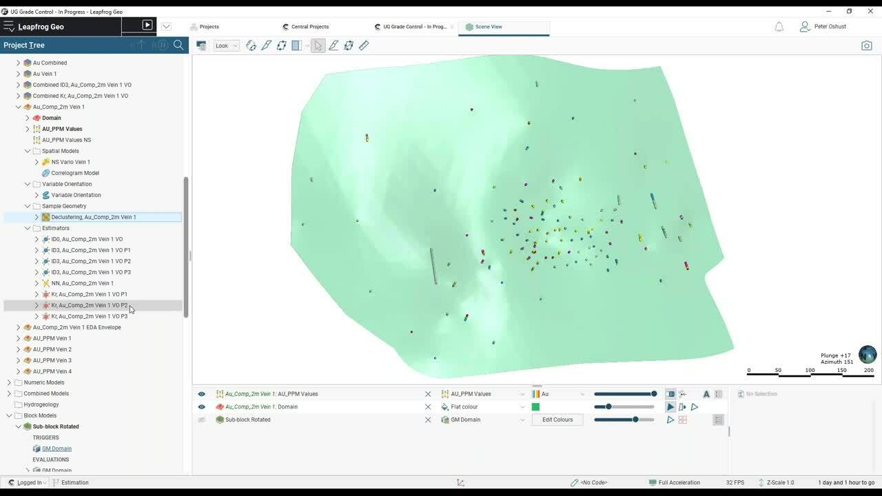
All right, now I’ll flip to the live demonstration.

[00:02:59.490]
And we’re starting off with a set of veins.

[00:03:04.430]
There are four veins here, quite a variety of drill holes,

[00:03:09.540]
not a lot of sapling, but that’s kind of common

[00:03:12.480]
with the many narrow vein situations

[00:03:14.790]
because it’s difficult to reach them.

[00:03:17.700]
Now let’s see what else we’ve got here.

[00:03:19.170]
So that’s all of our veins and all of the drill holes.

[00:03:23.040]
I’m going to load another scene,

[00:03:26.050]
which will show us what we’ve got for vein 1.

[00:03:30.290]
And it looks like I must have overwritten that scene.

[00:03:35.060]
So I’ll just turn off some of these other veins.

[00:03:38.350]
So here’s vein 1 with all of the drill holes.

[00:03:42.686]
So let’s filter some of these for vein 1.

[00:03:47.530]
So those are just the assays that we have in vein 1

[00:03:51.536]
and it’s pretty typical that we’ve got clustered data,

[00:03:54.586]
so they’ve really drilled this area off quite well

[00:03:56.280]
with some scattered holes out around the edge,

[00:04:00.622]
maybe chasing the extents of that structure.

[00:04:03.500]
So in other words, we’ve got some clustered data here.

[00:04:07.380]
So that’s a quick review of the data in the scene.

[00:04:10.830]
Now I’m going to flip to just looking at the sample lengths,

[00:04:15.970]
the assay interval lengths because those will help us

[00:04:19.860]
in making a decision on what composite length to use.

[00:04:23.140]
So this is the first of our EDA in the drill hole data.

[00:04:27.480]
And I’m going to go to the original assay table.

[00:04:32.590]
I do have a merged table that has the evaluated

[00:04:37.180]
geological model combined with the assays,

[00:04:39.750]
so we can do some filters on that.

[00:04:42.000]
But let’s just check the statistics on our table.

[00:04:45.640]
So at the table level, we have multivariate statistics

[00:04:49.009]
and we have access to the interval lengths statistics.

[00:04:52.800]
So looking at a cumulative histogram of sample lengths,

[00:04:56.720]
we can see that we have about 80% of the samples

[00:04:59.750]
were taken at one meter or less

[00:05:03.160]
and then about 20 are higher

[00:05:06.510]
and there’s quite a kick at two.

[00:05:10.286]
So it looks like, well, if we look at the histogram,

[00:05:11.930]
we’ll probably see the mode there,

[00:05:14.790]
a big mode at one,

[00:05:16.560]
but then it’s a little bumped down here at two meters.

[00:05:19.850]
So given that we don’t want to subdivide

[00:05:23.260]
our longer sample intervals,

[00:05:27.186]
which would impact the coefficient of variation, the CV,

[00:05:33.310]
it might make our data look a little bit better than it is,

[00:05:36.390]
so we’ll composite to two meters.

[00:05:39.340]
And that way we’ll get a better distribution of composites.

[00:05:47.110]
And we are expecting to see some changes,

[00:05:50.020]
but let’s look at what we’ve done for compositing.

[00:05:54.490]
I have a two-meter composite table here.

[00:05:56.600]
Just have a look at what we’ve done to composite.

[00:06:00.486]
So I’ve composited inside the evaluated GM,

[00:06:03.920]
that’s the back flag, if you want to think of it,

[00:06:05.620]
the back flag models, compositing to two meters.

[00:06:08.950]
And if we have any residual end lengths, one meter and less,

[00:06:14.220]
they get tagged or backstitched I should say,

[00:06:18.030]
backstitched to the previous assay intervals.

[00:06:20.450]
So that’s how we manage that

[00:06:22.441]
and composited all of the assay values.

[00:06:27.720]
So we have composites.

[00:06:30.220]
So let’s have a look at what the composites look like

[00:06:33.330]
in the scene then, I think I’ve got a scene saved for that.

[00:06:38.150]
No, I must have overwritten that one too.

[00:06:40.040]
I was playing on here this morning

[00:06:44.251]
and made a few new scenes,

[00:06:46.640]
I must have wrecked my earlier ones.

[00:06:48.970]
So let’s just get rid of the domain assays.

[00:06:54.690]
Click on the right spot and then load the composite.

[00:06:59.130]
So we have gold composites,

[00:07:02.990]
pretty much the same distribution.

[00:07:06.370]
And if I apply the vein 1 filter,

[00:07:09.080]
we’re not going to see too much different either.

[00:07:13.240]
Turn on the rendered tubes and make them fairly fat

[00:07:18.200]
so we can see what we’ve got here.

[00:07:20.591]
So there’s the composites.

[00:07:23.679]
Now we do have, again, that clustered data in here

[00:07:27.770]
and we have some areas where we had missing intervals

[00:07:32.840]
and now those intervals have been,

[00:07:36.150]
composite intervals have been created in there.

[00:07:38.140]
So I think the numbers of our composites have gone up,

[00:07:41.450]
but that’s a good thing really,

[00:07:43.790]
because we’ve got some low values in here

[00:07:45.990]
now that we can use to constrain the estimate.

[00:07:49.500]
Well, let’s just check the stats on our composites.

[00:07:57.210]
So we have 354 samples,

[00:07:59.890]
with an average of 1.9 approximately grams

[00:08:04.030]
and a CV of just over two.

[00:08:06.570]
So it does have some variants in this distribution

[00:08:11.910]
and it looks like we’ve got some outliers over here.

[00:08:16.690]
I did an analysis previously,

[00:08:18.540]
earlier on and I pegged 23 grams as the outliers.

[00:08:22.940]
If I want to see where these are in the scene

[00:08:25.440]
and you may know already that you can interact

[00:08:28.060]
from charts in the scene, it applies a dynamic filter.

[00:08:32.030]
So I’ve selected the tail in that histogram distribution,

[00:08:35.720]
and it’s filtered now for those composites in the scene

[00:08:38.920]
and I can see the distribution of them.

[00:08:42.299]
Now, if they’re almost clustered,

[00:08:43.550]
which means we might consider

[00:08:45.920]
using an outlier search restriction on these,

[00:08:48.440]
but I chose to cap them.

[00:08:50.680]
Generally speaking, if you have a cluster of outliers,

[00:08:53.630]
it may reflect the fact that there’s a subpopulation

[00:08:57.693]
that hasn’t been modeled out, so you can treat it

[00:08:59.927]
with a special outlier search restriction.

[00:09:05.090]
I’ll just get my vein 1 filter back here.

[00:09:08.950]
All right, so it was predetermined

[00:09:12.090]
that we would use vein 1 as a domain estimation.

[00:09:14.830]
So the next step in the workflow

[00:09:17.180]
is to add a domain estimation to our Estimations folder.

[00:09:22.740]
If you’re a Geo user, you won’t see estimations.

[00:09:26.710]
It’s only when you have the Edge extension

[00:09:28.460]
that you see this folder

[00:09:30.940]
where you can define the estimations

[00:09:33.420]
that you want to evaluate onto your block model.

[00:09:36.370]
So let’s just clear the scene on this one.

[00:09:39.760]
And I think I do have a scene ready to go for to this.

[00:09:43.980]
So let’s go to saved scenes.

[00:09:46.070]
Here’s my domain estimation using saved scenes,

[00:09:50.530]
just saves a few clicks.

[00:09:53.460]
Well, not a lot has changed from what we were looking at

[00:09:55.890]
in terms of composites, but you’ll see now

[00:09:59.369]
that where we had intervals in the drill holes before,

[00:10:01.820]
now we have discrete points.

[00:10:03.640]
So those reflect the centroids

[00:10:05.750]
or the centers of the composites.

[00:10:10.040]
And let’s have a look at, that’s the 3D view.

[00:10:13.910]
And let’s just check that the stats still look okay.

[00:10:17.750]
So go back up to the Estimation folder to the vein 1.

[00:10:23.320]
I guess I can show you what the boundary looks like too.

[00:10:26.930]
So I’m just double clicking on the domain estimation.

[00:10:30.930]
It’s calculating a boundary block

[00:10:33.930]
showing us the average grade inside the vein versus outside.

[00:10:39.170]
And what we’re paying attention to here

[00:10:40.940]
is what’s going on across the boundary.

[00:10:43.930]
And in this case, there’s quite a sharp drop in grade.

[00:10:47.040]
There’s a high grade contrast.

[00:10:49.250]
So I will use a hard boundary.

[00:10:51.450]
Now if this was more gradational,

[00:10:54.143]
if the boundary was a little bit fuzzy, for instance,

[00:10:55.850]
I could use a soft boundary and share samples

[00:10:59.300]
from the outside to a specified distance.

[00:11:02.656]
And this is calculated as perpendicular

[00:11:06.050]
to the triangle faces, so it’s nearly a true distance.

[00:11:09.900]
But I am going to use a hard boundary, just cancel that.

[00:11:14.600]
And we’ll start looking at some of the other things here.

[00:11:17.010]
So we’ve got the domain and the values loaded.

[00:11:19.830]
I also did a normal scores transform

[00:11:22.240]
in an effort to calculate a nicer variogram,

[00:11:27.030]
but in the end, I didn’t go there.

[00:11:30.425]
But we do have the ability to do

[00:11:32.370]
a Gaussian Weierstrass

[00:11:34.670]
or discreet Gaussian transformation,

[00:11:36.800]
whatever you want to call it.

[00:11:38.840]
Anyway, so it’s a normal scores transform,

[00:11:42.452]
which can sometimes help to improve modeling,

[00:11:45.740]
calculating and modeling variograms

[00:11:49.162]
in the presence of noisy data.

[00:11:50.890]
I opted instead, and we’ll go the correlogram here.

[00:11:54.810]
So we’re looking now at our spatial continuity in our model.

[00:11:59.190]
I opted to go with a correlogram

[00:12:02.130]
because a correlogram will work better

[00:12:06.150]
in the presence of clustered data.

[00:12:08.530]
It is very good at managing to control outliers, noisy data,

[00:12:14.250]
and it also helps to see past the clustered data.

[00:12:19.590]
So the correlogram, it’s the covariance function,

[00:12:24.810]
which has been normalized to the mean of the sample pairs,

[00:12:30.630]
if you want to think of it that way.

[00:12:32.190]
So the covariance function is divided by the,

[00:12:38.112]
the mean squared of the data or the standard deviation

[00:12:41.410]
of the data to normalize it to the mean.

[00:12:44.640]
So we can see in our map

[00:12:47.992]
that there is quite a strong vertical trend,

[00:12:50.810]
the pitch actually is the vertical

[00:12:53.820]
and the correlograms are displayed in their true form,

[00:12:57.610]
which is inverted to how we usually display

[00:13:01.500]
traditional semi-variograms.

[00:13:04.610]
Anyway, so that’s why these curves are upside down.

[00:13:07.400]
And I have managed to apply reasonable models, I think,

[00:13:11.430]
to the experimental variograms, so if we look in the scene,

[00:13:16.213]
we’ll see our variogram ellipse.

[00:13:20.300]
It’s not very big, so the continuity isn’t great.

[00:13:23.530]
But it does look reasonable together with the data.

[00:13:26.400]
So that is the go ahead variogram.

[00:13:31.920]
And the next thing we want to look at is declustering.

[00:13:35.460]
So clustered data will give you

[00:13:40.500]
typically an overstated naive mean of your samples.

[00:13:46.640]
So we use different declustering methods.

[00:13:49.590]
Leapfrog provides a moving window declustering.

[00:13:54.120]
You can also use a nearest neighbor model,

[00:13:56.440]
which gives you in effect like a 3D

[00:13:59.950]
polygonal volume type of a weighting.

[00:14:02.615]
So the samples are weighted by the inverse

[00:14:04.580]
of the area that they have around them.

[00:14:09.140]
And so these outline samples get more weight

[00:14:13.270]
than the closely spaced,

[00:14:15.940]
typically higher grade clustered data

[00:14:18.660]
where we’ve drilled off the higher grade

[00:14:20.660]
portion of the vein.

[00:14:22.980]
And so the declustered mean

[00:14:24.930]
is typically lower than your naive mean.

[00:14:29.190]
So let’s have a look if that’s the case

[00:14:30.690]
with our declustering tool in Edge.

[00:14:34.780]
So here’s our distribution.

[00:14:38.032]
And you can see as the moving window relative size

[00:14:41.290]
increases, that the average grade comes down

[00:14:45.360]
until it hits kind of a trough

[00:14:47.250]
and then it goes back up again.

[00:14:49.922]
And I suppose if you used a search ellipse

[00:14:52.632]
that was the same size as your vein,

[00:14:53.530]
it would come right back up to the input.

[00:14:56.640]
So the input mean, and this mean is a little bit different

[00:15:00.030]
than the 1.91 that we saw earlier.

[00:15:02.280]
So this is the mean of the points,

[00:15:06.332]
of the data rather than the length weighted intervals.

[00:15:08.360]
So it’s just slightly different,

[00:15:09.450]
but very close, 1.89, roughly.

[00:15:12.620]
And if I click on this node,

[00:15:14.740]
we’ll see that the declustered mean is 1.66.

[00:15:18.820]
So file that number away for later.

[00:15:23.490]
That’s our target.

[00:15:26.060]
Moving on to estimators,

[00:15:29.608]
and I defined three different estimators.

[00:15:32.890]
There’s an inverse distance cubed,

[00:15:35.700]
a nearest neighbor and a Creed estimator.

[00:15:40.707]
And with the CV up around two,

[00:15:42.230]
I was expecting that I would need

[00:15:44.000]
a slightly more selective type of an estimator

[00:15:46.940]
and that’s why IDCUBE.

[00:15:49.922]
And we’ll see what the results are comparing the Creed

[00:15:54.230]
to the inverse distance cubed.

[00:15:59.708]
Now I did a multi-pass strategy as well,

[00:16:03.106]
and that again, is to address the clustered data.

[00:16:06.520]
So the first pass search,

[00:16:08.360]
I’ll open up the first pass search here

[00:16:10.760]
using the variogram and the ellipsoid

[00:16:13.370]
is to the variogram limit.

[00:16:15.610]
So it looked reasonable as a starting point

[00:16:17.810]
for a first pass.

[00:16:20.545]
And I have set a minimum number of samples of 14

[00:16:24.100]
and a maximum of 20

[00:16:25.780]
and a maximum samples per drill hole of five.

[00:16:28.750]
That means that I need three holes on my first pass

[00:16:32.430]
to estimate a block.

[00:16:34.780]
And the block search isn’t very wide,

[00:16:38.490]
so I’m trying to minimize the negative Creeding weights.

[00:16:42.390]
So as the passes go, then the second pass uses a maximum

[00:16:48.330]
or two holes to estimate the block.

[00:16:51.760]
And then finally pass three, I’ll just show you,

[00:16:54.320]
is pretty wide open, big search

[00:16:57.530]
and no restrictions on the samples.

[00:17:00.831]
So even one sample will result in a block grade estimate.

[00:17:04.080]
So the idea here that this is just a fill pass,

[00:17:07.760]
making sure that as many blocks as possible are estimated,

[00:17:10.690]
and I use the similar strategies for the same sorry,

[00:17:15.390]
same search in sample selection for the IDCUBE.

[00:17:19.830]
So what does this look like when we evaluate it in a model?

[00:17:24.920]
Well, I guess first off, we’ll build a model.

[00:17:28.080]
Now I have one built already,

[00:17:30.322]
but as I mentioned, the kind of the trick

[00:17:32.480]
to doing the grade-thickness in Edge

[00:17:34.930]
is to define a rotated sub-block model.

[00:17:37.840]
So let’s see what that looks like.

[00:17:40.650]
A new sub-block model,

[00:17:44.530]
big parent blocks.

[00:17:45.530]
The parent blocks are scaled to the project limits

[00:17:49.870]
and it thinks that I need to have huge blocks

[00:17:53.880]
because the topography is very extensive,

[00:17:58.522]
but it’s not the case.

[00:17:59.420]
Now I’m going to use a 10 by 10 in the X and the Y

[00:18:03.240]
and the 300 in Z and when I’m done,

[00:18:06.450]
I will have the, well, the next step actually

[00:18:08.810]
is to rotate the model such that Z is across the vein

[00:18:13.950]
and that way, with a variable Z

[00:18:16.540]
going from zero to whatever it needs to be,

[00:18:19.440]
it will make like an array of blocks

[00:18:21.920]
that kind of look like little prisms.

[00:18:25.231]
There’s a shortcut to set the angles of a rotated model,

[00:18:29.070]
and that is to use a trend plane.

[00:18:30.860]
So let’s just go back to the scene,

[00:18:33.370]
align the camera up to look down dip of that vein

[00:18:39.542]
and I’ll just apply a trend plane here.

[00:18:42.280]
That’s got to be about 305.

[00:18:45.940]
I’m just going to edit this,

[00:18:47.795]
305 and the dip, 66 is okay.

[00:18:51.090]
I don’t need to worry about the pitch for this step.

[00:18:54.600]
It doesn’t come to bear

[00:18:56.730]
when I’m defining the block model geometry.

[00:18:59.460]
So now, I will set my angles from the moving plane.

[00:19:03.930]
And now that model, it’s a little bit jumped off

[00:19:08.900]
to the side there.

[00:19:11.045]
It is in the correct orientation now

[00:19:15.500]
at least for that vein, where am I?

[00:19:21.230]
Oh, my trend plane isn’t very good.

[00:19:23.000]
Let’s back up here.

[00:19:24.300]
I’m going to define a trend plane first

[00:19:31.382]
and then it’ll create a plane.

[00:19:34.292]
To the side, 305

[00:19:37.140]
and dipping, 66 I think was good enough.

[00:19:42.360]
Now a trend plane and let’s get back

[00:19:44.905]
to this block model business.

[00:19:46.380]
New sub-block model,

[00:19:50.402]
10 by 10 by 300.

[00:19:52.710]
I want to make sure that I go right across the vein

[00:19:55.410]
wherever there are any undulations.

[00:19:58.180]
And I will just have five-meter sub-blocks.

[00:20:01.490]
So the sub-block count two into 10

[00:20:05.070]
gives me my two five-meter sub-blocks

[00:20:09.830]
and let’s set angles from moving plane.

[00:20:15.890]
It’s better.

[00:20:16.780]
Now it’s lined up to where that vein is.

[00:20:19.455]
There’s a lot of extra real estate here that we can get.

[00:20:24.480]
We can trim that by moving the extents

[00:20:27.940]
a little bit back and forth.

[00:20:30.928]
Of course, the minimum thickness of that model

[00:20:34.030]
in the Z direction is going to be 300

[00:20:36.370]
because that’s what I have set my Z dimension to be.

[00:20:43.530]
One more tweak and that’s roughed in pretty, pretty good.

[00:20:50.640]
Of course, if you had an open pit,

[00:20:51.990]
you would have to make it a little bit bigger,

[00:20:54.630]
but this is going to be an underground mine.

[00:20:57.270]
So that’s aligning it to the model

[00:21:00.830]
and you can see by the checkerboard pattern

[00:21:03.090]
that Z is across the vein.

[00:21:06.327]
And then after that, I would set my sub-blocking triggers

[00:21:07.960]
and devaluations and carry on.

[00:21:10.670]
Now we already have a model built.

[00:21:12.410]
So I’ll just click Cancel at this point

[00:21:16.735]
and bring that model into the scene.

[00:21:19.805]
Well, the first thing we could look at

[00:21:21.720]
is the evaluated geological model.

[00:21:25.010]
Oops, the evaluated geological model

[00:21:29.070]
and that is filtered for measured and indicated blocks,

[00:21:31.940]
but there’s the model.

[00:21:35.739]
And if we cut a slice right along the model trend

[00:21:41.060]
slice and cross the vein

[00:21:47.700]
and then set the width to five and the step size to five.

[00:21:52.770]
And this can be 125.

[00:21:55.820]
Now I am looking perpendicular to the model.

[00:22:00.440]
And if I hit L, on the keyboard to look at that model,

[00:22:07.040]
I should be able to see those prisms

[00:22:09.840]
that I was looking for.

[00:22:10.890]
Yeah, they’re all kind of prisms.

[00:22:12.540]
We can see this model isn’t very thick or tall,

[00:22:15.280]
it’s only about five meters or less.

[00:22:19.940]
And I don’t see any breaks in the block.

[00:22:22.290]
So that means that my Z value at 300 is pretty good.

[00:22:26.260]
If I would have used a Z at, let’s say a 100 meters,

[00:22:29.780]
I may have had some blocks being split,

[00:22:32.300]
but I want only blocks that are completely across

[00:22:36.454]
that vein in the Z direction.

[00:22:40.960]
So let’s turn off these lights, we’ve got our model

[00:22:44.360]
and of course we’ve evaluated the GM

[00:22:47.560]
and I set the sub-blocking triggers to the GM as well.

[00:22:51.890]
Now I’m just going to my cheat sheet here

[00:22:53.750]
to see what I also want to show you.

[00:22:56.580]
So at this point, yeah,

[00:22:58.239]
let’s have a quick look at some of the models.

[00:23:00.560]
So that’s the geology.

[00:23:04.060]
I evaluated,

[00:23:05.360]
I created, sorry, I created a combined estimator

[00:23:08.170]
for the three passes for the inverse distance cubed

[00:23:12.040]
and the Creed estimator

[00:23:13.900]
so that I can combine all three passes.

[00:23:16.810]
Actually, I better show you what that looks like.

[00:23:19.180]
So in the combined estimator,

[00:23:21.410]
I just double clicked on it to open.

[00:23:23.320]
I selected passes one, two, and three in order.

[00:23:26.528]
It’s important because as a block is estimated,

[00:23:30.930]
it doesn’t get overwritten by the following passes.

[00:23:34.700]
So if I were to put pass three at the top,

[00:23:37.160]
of course, everything would have been estimated

[00:23:38.680]
with pass three and pass one and two

[00:23:40.610]
wouldn’t have had any impact on the model at all.

[00:23:43.130]
So yes, hierarchy is important and it is correct.

[00:23:48.210]
So let’s just have a look at that model.

[00:23:51.690]
So there’s the Creed, here’s the Creed model

[00:23:55.745]
and it’s not bad, but I can see,

[00:23:59.420]
I would have to tune it a little bit better.

[00:24:01.410]
I think there’s some funny artifact patches of blocks

[00:24:04.870]
and things, may or may not be able to get rid of those.

[00:24:11.520]
And there are big areas around the edge

[00:24:15.370]
that have just one grade.

[00:24:17.480]
So that’s kind of reflecting

[00:24:19.518]
the fact that there’s not a lot of data out there

[00:24:21.180]
and that third pass search basically estimating the block

[00:24:24.490]
with that one pass.

[00:24:26.670]
Let’s see what the IDCUBE model looks like.

[00:24:31.000]
That’s a much prettier model, I guess

[00:24:33.430]
because the thing is how does it validate?

[00:24:37.195]
And we will check it against the nearest neighbor model,

[00:24:40.750]
which is kind of a proxy to a declustered distribution.

[00:24:44.150]
Even though we will have more than one sample per block,

[00:24:48.280]
it does kind of emulate or is a proxy for

[00:24:52.343]
properly declustered to distribution.

[00:24:55.990]
Anyway, let’s go back to the IDCUBE.

[00:24:59.260]
Another thing that we can do,

[00:25:01.330]
and that is to restrict our comparison

[00:25:06.490]
within a reasonable envelope

[00:25:08.870]
around the blocks that are well-supported.

[00:25:14.042]
So this is basically, where does it matter?

[00:25:15.980]
Like it doesn’t matter so much around the edges,

[00:25:18.580]
we’re expecting a little bit of error out there.

[00:25:24.795]
But if we define a boundary

[00:25:27.010]
around that are of the well-drilled region,

[00:25:35.360]
and it’s showing in there.

[00:25:38.190]
There’s my well-drilled region.

[00:25:39.550]
So I’m calling this my EDA envelope.

[00:25:42.050]
I’m going to do my validation checks in that envelope.

[00:25:45.955]
They’re going to be much more relevant

[00:25:48.745]
than just having everything on the outside

[00:25:51.870]
that is inferred confidence or less, let’s say.

[00:25:55.720]
Okay, back to the model and let’s check our stats.

[00:26:01.090]
So going to check statistics, table of statistics.

[00:26:07.505]
And I want to replicate the mean of the distribution

[00:26:13.500]
with my estimates.

[00:26:14.920]
And you’ll recall that the declustered mean is 1.66,

[00:26:19.845]
the nearest neighbor model is also very close to that

[00:26:22.600]
within a percent, 1.689, and the CV is almost the same

[00:26:28.240]
as it was for our samples, which was two.

[00:26:30.982]
So that nearest neighbor model,

[00:26:33.116]
again, reasonable proxy

[00:26:35.550]
for the declustered grade distribution

[00:26:37.970]
and very useful for comparison.

[00:26:40.040]
The IDCUBE model comes in quite well.

[00:26:43.960]
Well, it’s a little bit off, but not bad, 1.73, roughly.

[00:26:47.400]
So we’re replicating the mean of our input distribution

[00:26:52.530]
with the IDCUBE.

[00:26:54.530]
For some reason, we’ve got higher grades

[00:26:57.470]
in the ordinary Creed model than we do in our samples.

[00:27:02.450]
So that’s kind of a warning sign

[00:27:05.000]
and it is very much smoothed,

[00:27:06.810]
it’s .65, a CV of .66, which is much less than two,

[00:27:11.800]
so it’s probably overly smoothed.

[00:27:14.290]
And without doing any additional validation checks,

[00:27:17.280]
I’m going to use my IDCUBE as the go-ahead model

[00:27:21.160]
and yeah, carry on from there.

[00:27:26.240]
Now let’s see.

[00:27:27.220]
Oh, I didn’t mention it,

[00:27:28.932]
but yeah, I did do variable orientation.

[00:27:31.810]
Funny how you can miss stuff when you’re doing these demos.

[00:27:36.270]
I did do a variable orientation,

[00:27:38.730]
which is using the vein to capture the dynamic

[00:27:44.720]
or locally varying iroinite in the estimation,

[00:27:49.440]
our implementation of variable orientation in Edge

[00:27:53.450]
changes the direction of the search

[00:27:55.980]
and the direction of the variogram,

[00:27:57.480]
it doesn’t recalculate the variogram.

[00:27:59.200]
It just changes the directions

[00:28:01.120]
and applies that to the search

[00:28:02.980]
so that we get a much better local estimate

[00:28:06.750]
using the variable orientation.

[00:28:09.400]
Okay, so moving right along,

[00:28:12.818]
and the next thing is to get into the calculations

[00:28:15.600]
because that’s where we do the grade-thickness.

[00:28:18.390]
So I’m going to double-click on Calculations,

[00:28:21.030]
it’ll open up my calculations editor.

[00:28:23.540]
I better show you the

[00:28:29.910]
panel with the tools

[00:28:32.600]
Where are my tools?

[00:28:36.660]
I’ll maybe open it in another way here.

[00:28:41.455]
‘Cause I have to show you that panel.

[00:28:42.950]
Calculations and filters

[00:28:53.082]
so there should be a panel that pops out here

[00:28:56.280]
that we can see the metadata that is used

[00:29:01.450]
or the items we can select, go into the calculations

[00:29:04.450]
and our syntax buttons.

[00:29:08.342]
And isn’t that funny?

[00:29:09.953]
It’s not being active for me.

[00:29:10.950]
Well, let’s have a look at the calculations anyway,

[00:29:12.770]
because the syntax is sort of self-explanatory.

[00:29:16.670]
So I did do a filter for the,

[00:29:21.010]
let’s expand, collapse that.

[00:29:23.092]
So I did do a filter for my measured in indicated,

[00:29:25.970]
which is within the EDA envelope.

[00:29:28.920]
So that was my limits.

[00:29:31.360]
I also did some error traps that found empty blocks

[00:29:37.470]
and put in a background value.

[00:29:39.140]
They didn’t get estimated.

[00:29:41.055]
So if it’s the vein and the estimate is normal,

[00:29:44.320]
then it gets that value,

[00:29:45.620]
otherwise it gets a low background value.

[00:29:48.030]
And I did that for each of my models.

[00:29:50.850]
I also calculated a class, category calculation for class.

[00:29:56.450]
So if it was in the vein and it was in the EDA envelope,

[00:30:00.610]
and within 25 meters, then it gets measured,

[00:30:02.940]
otherwise in the EDA envelope, it’s indicated.

[00:30:06.090]
So I did contour

[00:30:09.990]
the region of 25 to 45 meters

[00:30:14.860]
and then drew a poly line.

[00:30:17.110]
And that was what formed my EDA envelope.

[00:30:20.010]
And then outside of that, if it’s inferred

[00:30:23.310]
or if it’s still in the vein

[00:30:25.030]
but beyond the indicated boundary,

[00:30:28.677]
or my EDA envelope, then I just called it inferred.

[00:30:33.670]
So there’s also, I did for the statistics,

[00:30:39.390]
I did also create calculated,

[00:30:44.360]
numeric calculation of the measured and indicated blocks,

[00:30:49.060]
two those were just for more comparisons.

[00:30:51.900]
But finally, finally, we’re getting to the thickness.

[00:30:55.490]
So the thickness is pretty straightforward

[00:30:57.050]
because we have access to the Z dimension.

[00:31:01.000]
So all I had to do for thickness

[00:31:03.230]
is say, if it was in the vein,

[00:31:05.230]
then give the thickness model the value of the Z dimension,

[00:31:09.530]
otherwise it’s outside.

[00:31:11.620]
And then the next step after that

[00:31:14.350]
is to do a calculation, very simple.

[00:31:18.170]
If that block was normally estimated has a value,

[00:31:20.780]
in other words, then we just multiply our thickness

[00:31:24.230]
times the grade of that final model.

[00:31:26.330]
And I used the IDCUBE model, and that’s that.

[00:31:30.170]
So we can then look at these models in the scene.

[00:31:37.100]
Any calculation that we do can be visualized in the scene.

[00:31:40.460]
So let’s have a look there, see the thickness,

[00:31:42.820]
so you can see where there might be some shoots

[00:31:47.620]
in that kind of orientation.

[00:31:51.435]
And if we multiply, sorry, grade times thickness,

[00:31:56.400]
we can see, yeah, maybe there are some shoots

[00:31:59.280]
that we need to pay attention to,

[00:32:01.870]
maybe target some holes down plunge of these shoots

[00:32:06.530]
to see exactly what’s going on.

[00:32:10.084]
And as I mentioned, that model exists,

[00:32:14.280]
well exists, we can now export that model

[00:32:18.780]
to give it to the engineers.

[00:32:21.490]
So let’s just go to our model.

[00:32:24.500]
What does that look like?

[00:32:26.350]
Export,

[00:32:29.260]
let’s call it Sub-block Model Rotated,

[00:32:33.550]
and we can export just the CSV file

[00:32:36.480]
that has all of the information in top of the file,

[00:32:42.740]
a CSV with a separate text file for that metadata,

[00:32:46.110]
or just points if you just need the points

[00:32:48.460]
for maybe contouring or something,

[00:32:51.010]
but I’m going to select that CV output format.

[00:32:56.037]
Well, I’ve already done this, so it is somewhat persistent.

[00:32:59.670]
It remembered which models I had exported

[00:33:03.500]
and then applying a query filters

[00:33:06.210]
so I’m not exporting the entire model,

[00:33:08.650]
just the one for vein 1

[00:33:10.910]
and ignoring rows or columns

[00:33:14.730]
where all of the blocks were in air condition or empty.

[00:33:18.170]
And then I can use status codes, either his texts

[00:33:22.135]
or his numerics, carry on here

[00:33:26.100]
and pick the character set.

[00:33:27.260]
The default usually works here in North America,

[00:33:31.687]
and there’s a summary and finally export.

[00:33:33.440]
There aren’t a lot of blocks there,

[00:33:34.570]
so the export actually happens pretty quickly.

[00:33:37.970]
So let me see what else I’ve got here.

[00:33:44.130]
Yes, okay, so the filter,

[00:33:46.417]
I just want to show you in the block model,

[00:33:48.290]
I did define that filter for the vein

[00:33:50.980]
1 measured and indicated.

[00:33:53.250]
So that is kind of the view again,

[00:33:56.400]
where the blocks are filtered for what matters.

[00:34:00.210]
And that’s actually is, that’s the workflow.

[00:34:03.740]
And I hope I’ve covered it in 30 minutes or less,

[00:34:07.970]
and the floor is now open for questions.

[00:34:13.010]
<v Hannah>Awesome, thanks, Peter.</v>

[00:34:13.843]
That was really good.

[00:34:15.670]
I even learned a couple of things.

[00:34:18.504]
I love when you sprinkle breadcrumbs of knowledge

[00:34:22.050]
throughout your demos.

[00:34:24.240]
Right, so we’ve got some time for questions here.

[00:34:26.220]
I’ll give everybody a moment to type some things

[00:34:30.530]
into that questions panel, if you haven’t done so already.

[00:34:35.010]
I’ll start, Peter, there’s a couple of questions here.

[00:34:39.267]
So the first one,

[00:34:41.217]
how can you view sample distance on a block model?

[00:34:46.480]
<v Peter>Okay, maybe I’ll go back to Leapfrog</v>

[00:34:49.850]
for that then.

[00:34:51.330]
So sample or average distance and minimum distance

[00:34:56.000]
are captured in the estimator.

[00:34:57.830]
So let’s just go up to an estimator.

[00:35:07.217]
Estimator, I’ll use the combined one.

[00:35:09.314]
And in the outputs tab, if I want to see the minimum

[00:35:11.410]
or average distance, I can select those

[00:35:14.140]
as the output number of samples as well.

[00:35:18.354]
So with that one selected,

[00:35:20.104]
I should be able to go to my evaluated model.

[00:35:24.660]
There’s my combined ID3 estimator, there’s average distance.

[00:35:29.637]
So there’s a map of distance, to samples

[00:35:35.690]
and each block, if I click on a block,

[00:35:38.070]
I can actually go right to the absolute value.

[00:35:42.060]
And you can export this too if you need that kind of thing

[00:35:46.400]
in the exported block model.

[00:35:49.850]
<v Hannah>Okay, thanks, Peter.</v>

[00:35:52.140]
Another question,

[00:35:53.210]
how can I find that grade-thickness workflow

[00:35:57.900]
on drill holes?

[00:36:00.150]
I can actually just paste that into the chat here.

[00:36:02.800]
I’ll paste that hyperlink.

[00:36:05.910]
So that was our, we had a Tips &amp; Tricks session

[00:36:08.150]
as part of our Lyceum. I’ll put that in the chat here.

[00:36:12.660]
Okay, another question,

[00:36:13.780]
we saw you pick your declustering distance in the plot.

[00:36:20.501]
Is this typically how all

[00:36:21.520]
<v Peter>I missed the question Hannah.</v>

[00:36:23.414]
<v Hannah>We saw you pick your declustering distances</v>

[00:36:27.120]
or distance in the plot, is that typically how

[00:36:30.010]
all declustering distances are selected

[00:36:32.100]
or can you speak more about declustering distances?

[00:36:36.400]
<v Peter>Well, generally speaking,</v>

[00:36:39.080]
when we’re doing declustering,

[00:36:40.760]
we’re targeting distribution

[00:36:44.750]
where the area of interest has been drilled off more

[00:36:49.537]
than outside and consequently,

[00:36:52.120]
the naive average is higher than the declustered average.

[00:36:57.410]
So that’s why I’m picking the lowest point here,

[00:37:01.940]
the lowest mean from the moving window relative size.

[00:37:08.920]
And so it’s,

[00:37:12.464]
now that isn’t always the case.

[00:37:13.490]
It could be flipped if you’re dealing with contaminants.

[00:37:16.250]
In that case, you might find that your curve is upside down

[00:37:20.610]
or inverted with respect to this one,

[00:37:22.680]
and you would pick the highest one.

[00:37:25.080]
So I have seen that a couple of times.

[00:37:26.880]
I don’t have a dataset that I can emulate that,

[00:37:31.514]
but this is typically where you’re picking

[00:37:34.735]
your decluttering mean.

[00:37:36.160]
Did that answer the question?

[00:37:37.840]
<v Hannah>I think so, yeah.</v>

[00:37:38.910]
<v Peter>Okay.</v>

[00:37:40.426]
<v Hannah>Another question just came in.</v>

[00:37:42.330]
I know we’re past our time here,

[00:37:44.170]
but I do want to squeeze these out

[00:37:46.210]
for anyone who’s interested so.

[00:37:47.770]
Thanks, great presentation.

[00:37:49.370]
Is there a limitation to the model size

[00:37:51.980]
for import or export using Edge?

[00:37:55.887]
I guess we mean block model there.

[00:37:57.410]
<v Peter>Yeah, there doesn’t appear to be a hard limit</v>

[00:38:01.987]
on most block sizes.

[00:38:04.010]
However, I should qualify that the current structure

[00:38:07.875]
for the Edge block model does not support

[00:38:11.120]
the importing of sub-block models.

[00:38:13.980]
So while you can export a sub-block model,

[00:38:15.980]
you can’t import one, which is a bit of a limitation

[00:38:18.660]
until we fully implement the octree structure,

[00:38:22.210]
which is similar to some of what our competitors

[00:38:26.727]
that use sub-blocked models as well.

[00:38:29.827]
But I know there are people out there

[00:38:31.850]
that have billion blocked block models

[00:38:35.277]
that they’re working actively within their organizations,

[00:38:38.740]
mind you they’re very cumbersome at that scale.

[00:38:43.490]
<v Hannah>Right, okay.</v>

[00:38:47.090]
Well, that wraps up our questions.

[00:38:50.480]
We’ve got another one who says thank you.

[00:38:52.787]
You’re welcome.

[00:38:53.620]
So thanks again, Peter.

[00:38:54.825]
That was awesome.

[00:38:56.614]
(gentle music)