Innovative integrated exploration approach for geothermal reservoirs, a case study from the Netherlands

The energy transition in the Netherlands requires a sustainable and renewable supply of heat besides electricity that at present is still largely provided by fossil energy sources. Their integrated workflow makes use of proven and established exploration techniques and has been key in making the energy transition in the Netherlands but is also relevant in regions which are currently still under-explored.

Video Transcript

[00:00:00.391](upbeat music)

[00:00:10.070]<v Sean>Welcome everybody.</v>

[00:00:10.903]Good afternoon and thanks for joining us

[00:00:12.692]for today’s webinar.

[00:00:15.490]Just as a quick introduction my name’s Sean Goodman.

[00:00:18.460]I’m one of Seequent regional segment managers

[00:00:21.100]covering energy across the Emir Region.

[00:00:24.300]So I’m happy to be joined by Peter van Heiningen

[00:00:28.930]and Vincent van Hoegaendan.

[00:00:32.189]I’m sorry I’ve just butchered that.

[00:00:34.047]<v Vincent>Yeah, no problem.</v>

[00:00:36.361]<v Sean>Who are the co-founders and directors</v>

[00:00:38.050]of Blue Gold Exploration Consultancy based

[00:00:40.530]in the Netherlands.

[00:00:41.790]So today there’ll be taking us through

[00:00:43.790]the integrated geothermal exploration workflow,

[00:00:46.940]which makes use of established exploration techniques.

[00:00:50.300]And there’ll be presenting a case study

[00:00:51.970]from the Netherlands but the workflow

[00:00:53.650]is also relevant in other regions around the world,

[00:00:56.270]which are currently still under explored.

[00:00:59.320]So Peter is a principal geologist.

[00:01:02.660]He’s got over 25 years experience and knowledge within

[00:01:07.000]the worldwide exploration for natural resources.

[00:01:09.770]He has been applying this experience to exploration

[00:01:12.540]for medium to high temperature geothermal energy

[00:01:14.980]for the last 10 years.

[00:01:17.176]Having graduated in geology from Utrecht University in ’97,

[00:01:22.450]he’s a member of EAG, AAPG, and the IGA

[00:01:27.600]and a member of the board of stakeholders

[00:01:29.200]for European Technology and Innovation Platform

[00:01:31.810]on deep geothermal.

[00:01:33.900]He’s previously worked at Schlumberger, CGG-Fugro, Gulf,

[00:01:37.360]and at the VU and the ITC.

[00:01:40.580]Vincent is a principle geophysicist at Blue Gold

[00:01:44.380]with a career spanning more than 30 years at Shell,

[00:01:47.820]CGG-Furgo, RPS, as well as TNO, Ecofys, and Alliander.

[00:01:52.980]He’s split his time approximately 50% in fossil fuels

[00:01:56.570]and 50% in renewable energy and graduated in physics

[00:02:00.480]from Utrecht University in 1986.

[00:02:03.494]He’s a member of EEG for geological risk production

[00:02:08.040]in deep geothermal exploration projects.

[00:02:10.730]He’s developed Blue Gold’s

[00:02:12.800]proprietary SeismoLog PRO technology

[00:02:15.550]and software which we’ll be hearing more about today.

[00:02:19.020]So Peter, Vincent, I thank you for joining us today

[00:02:22.820]and it’s over to you if you’d like to crack on.

[00:02:26.050]<v Vincent>Yeah, thank you very much, Sean,</v>

[00:02:28.810]for your introduction.

[00:02:30.570]It’s a pleasure for us to…

[00:02:34.660]Peter and I to talk about

[00:02:36.940]this innovative, integrated exploration approach

[00:02:40.370]for a geothermal reservoirs

[00:02:42.480]and we’re happy to share with you a case study

[00:02:45.410]from the Netherlands, actually from Amsterdam.

[00:02:48.820]Please, next slide.

[00:02:53.605]As Sean has talked about already Peter and I

[00:02:57.200]we have founded our company,

[00:03:01.550]Blue Gold Exploration Consultancy this year,

[00:03:05.070]working upon work that we’ve done already for several years

[00:03:09.590]in geothermal energy.

[00:03:12.750]Our coworkers, our associates are,

[00:03:16.000]Professor Kaymakci who is a structural geologist

[00:03:20.770]from Turkey and to Dr. Tijmen Jan Moser

[00:03:24.510]who’s a very experienced seismic processor working

[00:03:28.390]upon others at various techniques

[00:03:31.390]to get more fault information out of seismic data.

[00:03:37.040]Please, the next slide.

[00:03:39.770]What is the contents of our presentation?

[00:03:42.210]First of all, we will show you the objective.

[00:03:45.610]Then the current status and structuration

[00:03:48.370]of deep geothermal projects in the Netherlands.

[00:03:51.860]We will show you the data sets

[00:03:53.630]that we will use in our case study, namely Amsterdam.

[00:03:59.010]We will show details of our unique workflow

[00:04:03.160]with a special focus Seismolog PRO

[00:04:06.070]our unique correction method for density and velocity logs.

[00:04:12.380]Then we will show the seismic to well match a few things

[00:04:17.020]about the geological setting

[00:04:18.410]because the main focus of this presentation

[00:04:21.880]is really on Seismolog PRO and GravMag work.

[00:04:27.840]And then Peter will talk more

[00:04:31.840]about gravity and magnetics interpretation and modeling.

[00:04:36.830]And after that, we will come up with our summary

[00:04:39.960]and conclusions.

[00:04:41.550]Next slide, please.

[00:04:44.230]Okay, what is the objective of our webinar?

[00:04:47.990]We really would like to demonstrate

[00:04:49.970]you the successful application of gravity and magnetics data

[00:04:54.420]in mapping deep geothermal prospects using the sequence,

[00:04:59.150]Geosoft software for that

[00:05:01.220]but also our own proprietary SeismoLog PRO software.

[00:05:06.360]And the example is as explained earlier about

[00:05:09.770]the nice City of Amsterdam.

[00:05:12.860]Next slide, please.

[00:05:20.350]Yeah, I hope it’s visible for the order

[00:05:26.500]or the answer or the world.

[00:05:28.980]We show you here on the left.

[00:05:30.630]We show you the map of the Netherlands

[00:05:34.070]and the green areas actually indicate geological,

[00:05:40.450]sorry, geothermal exploration projects.

[00:05:44.550]The study area,

[00:05:45.950]which is indicated as the red rectangle

[00:05:50.150]is the Amsterdam area where we will talk about more.

[00:05:54.450]And you can see already

[00:05:55.560]that there is quite lively exploration already going on

[00:06:00.140]in terms of geothermal energy in the Netherlands.

[00:06:04.520]The phasing of geothermal energy projects

[00:06:08.900]is shown on the right hand side.

[00:06:12.650]You see here, phase zero and phase one,

[00:06:15.310]that is in general…

[00:06:17.200]These are in general, the real exploration activities

[00:06:23.030]that lead to the actual attainment of a permit,

[00:06:29.550]expiration permit.

[00:06:32.040]Phase two are the preparation activities

[00:06:36.760]for actually going forward

[00:06:39.400]with the drilling of an exploration well.

[00:06:43.810]And in the case of geothermal energy

[00:06:45.540]that’s normally drilling two wells.

[00:06:48.300]Yeah, so phase three, as we call it

[00:06:51.740]in the Netherlands for reduce thermal project

[00:06:54.490]is in general after the wells have been drilled,

[00:06:58.710]you get maintenance,

[00:07:00.610]you probably need some extra wells in the whole area

[00:07:04.770]to be drilled, so that’s phase three.

[00:07:07.450]And just to give you a good indication of the investments

[00:07:11.090]that you do in each phase.

[00:07:13.270]Let’s say the first phase, phase one,

[00:07:15.260]you generally spent something like €100,000.

[00:07:19.600]In phase two, you have to spend up to €500,000

[00:07:27.950]if possible for seismic data.

[00:07:31.740]If the seismic data is already there, for instance,

[00:07:34.280]you have the 3D seismic data set, you don’t really need it.

[00:07:38.430]And phase three, the drilling of the wells,

[00:07:43.490]that’s actually the most intense investment phase

[00:07:49.850]where you have to spend €15 to €20 million

[00:07:54.040]for drilling two geothermal wells.

[00:07:57.780]Next slide, please.

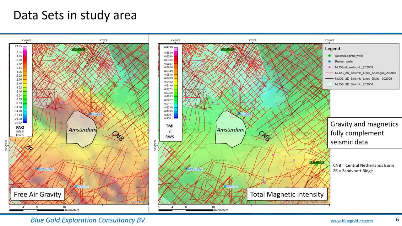
[00:08:05.610]Yeah, the study area, Amsterdam, as we talked about.

[00:08:11.230]What you see here in these two colorful pictures

[00:08:15.924]as background color.

[00:08:17.850]The free air gravity measurement that has been done over

[00:08:22.120]the whole of the Netherlands.

[00:08:24.000]And on the right-hand side you see in the background color,

[00:08:28.810]you see the total magnetic intensity.

[00:08:32.540]The area of Amsterdam is indicated in the middle part

[00:08:37.290]and what you see as red lines are actually

[00:08:40.537]the 2D seismic lines that have been shot in the past

[00:08:45.240]for oil and gas exploration.

[00:08:47.810]And, as you can see, the area of Amsterdam

[00:08:51.650]is actually not covered at all with seismic lines,

[00:08:56.161]which is actually a problem for other geothermal operators

[00:09:03.800]that are only costumed to interpreting seismic data.

[00:09:08.410]So that’s really also the reason why we have chosen

[00:09:11.380]this Amsterdam area for this webinar

[00:09:14.250]to show you what GraVMag data

[00:09:17.380]and the interpretation of that can actually bring you

[00:09:20.690]what’s in this area.

[00:09:22.000]Seismic data can not bring you at all.

[00:09:25.510]Next slide, please.

[00:09:29.930]What is our workflow?

[00:09:31.440]Our workflow is actually centered around getting

[00:09:34.830]the hard data, the lock data, density,

[00:09:38.500]and velocity data completely up to standards,

[00:09:44.070]high standards, and bringing in check shell data,

[00:09:48.530]bringing in the lishtology data

[00:09:50.850]and actually to come up with logs, velocity,

[00:09:53.700]and density logs that are complete and consistent

[00:09:57.890]with each other from surface down to TD.

[00:10:01.803]That really are the main part of all our work.

[00:10:06.220]The SeismoLog PRO work flow.

[00:10:09.260]And that information, so, for instance,

[00:10:11.640]the velocity information is actually

[00:10:13.440]then used in the seismic reprocessing

[00:10:16.920]what you can see on the upper right-hand side

[00:10:20.840]for depths migration, but also for time

[00:10:25.410]to depths conversion.

[00:10:29.640]The second thing, which is also a unique thing

[00:10:32.610]that we use in this workflow

[00:10:35.890]is the GravMag interpretation,

[00:10:38.600]which builds upon the robust density logs

[00:10:43.160]that are made by us from surface down to TD.

[00:10:47.480]And that allows us to model in a 2D sense,

[00:10:52.880]the various horizons in the area of interest.

[00:10:58.620]So what you see on the left-hand side as text

[00:11:03.980]is really that our workflow pivots around

[00:11:08.300]the SeismoLog PRO proprietary software

[00:11:11.860]but also the SEEQUENT-Geosoft software.

[00:11:18.700]In this workflow, we spent this amount of work also

[00:11:26.020]because we see that when you can de-risk

[00:11:30.278]the geology and actually really find

[00:11:34.920]the prospects, the geothermal prospects,

[00:11:39.210]and get a good handle on the density, but also the porosity

[00:11:43.820]you can actually de-risk your projects

[00:11:46.200]from say a success ratio of only 25% up to 75%,

[00:11:53.600]which for a drilling project of €20 million

[00:11:58.150]is really worthwhile.

[00:12:02.820]The second thing, what is the advantage of our workflow

[00:12:06.830]is that we do not only depend on seismic data.

[00:12:12.300]We also use the GravMag data.

[00:12:14.470]We are able to actually uncover the geology

[00:12:20.320]in areas like the Amsterdam area,

[00:12:23.660]where there is no seismic data at all.

[00:12:27.450]Next slide, please.

[00:12:31.990]Then a few words on SeismoLog PRO.

[00:12:35.730]You see here on the left, in the graph,

[00:12:39.460]you see a SeismoLog PRO exercise on a well

[00:12:43.640]that we have used for this incident study.

[00:12:47.790]As the red curve, this indicates actually

[00:12:51.540]the result of this workflow.

[00:12:56.780]As you can see, the red curve starts

[00:12:59.860]from the surface which is above

[00:13:03.960]and it goes all the way down TD, total depths of the well.

[00:13:10.090]What you can see in the shallow part is actually

[00:13:13.100]that it fills in the whole area which is actually lacking

[00:13:17.770]in the black curve.

[00:13:20.120]The black curve is namely the raw curves that are available

[00:13:26.640]in the online TNO database for logs that have been logged

[00:13:33.520]for the oil and gas Wells.

[00:13:36.450]As you can see also that there are quite some discrepancies

[00:13:41.070]between the black curve, which is raw curve

[00:13:46.060]and the SeismoLog PRO curve.

[00:13:49.170]And what you can see is that there are various areas

[00:13:53.625]where they differ, where they are actually improved.

[00:13:59.220]Not only do we actually make a good synthesis

[00:14:04.180]between the lithology and the logs

[00:14:07.920]but we also bring in the check shot data.

[00:14:11.780]So the check shot data, which is very valuable data

[00:14:16.150]is used to derive interval philosophies using

[00:14:22.201]our own methods and also ray tracing.

[00:14:30.440]Please, the next slide.

[00:14:35.640]Here, you see the results

[00:14:37.050]because we do the SeismoLog PRO work not only

[00:14:39.534]on the velocity data but also on the density data.

[00:14:43.470]And you see here, quite a significant change in the results

[00:14:48.950]of the SeismoLog PRO for the density.

[00:14:51.970]The density namely is in the middle part of this log,

[00:14:58.030]completely improved and slow down in terms of value.

[00:15:06.550]So it has been decreased in value based

[00:15:09.870]on the synthesis of both the velocity and the density

[00:15:16.730]that it has to conform to a certain lithology,

[00:15:19.890]which is actually found in the lithology.

[00:15:23.020]So what we found out in this exercise

[00:15:25.710]is that the density log which is the role density log,

[00:15:29.530]which is shown here in black is actually far too high due

[00:15:35.340]to the fact that it was actually locked

[00:15:38.470]in the casing itself.

[00:15:40.430]So we had to derive various lithology dependent relations

[00:15:45.320]between velocity and density to come up with the right

[00:15:49.330]and correct density.

[00:15:52.140]Many people often look only at the velocity logs

[00:15:56.890]when they have assessment project,

[00:15:59.630]but since we are also doing GravMag data,

[00:16:03.300]this relies very heavily on the density information

[00:16:07.290]of the various formations.

[00:16:10.110]So that’s why this SeismoLog PRO work

[00:16:12.600]is essential also for the GravMag work

[00:16:15.470]to function in the right way.

[00:16:18.550]As you can see at the lower hand side

[00:16:21.780]of the blocks you see.

[00:16:24.490]In fact, the rotliegend sandstone

[00:16:27.700]which is in this area also the reservoir

[00:16:31.870]for the geothermal heat.

[00:16:35.070]Next slide, please.

[00:16:40.100]Then as people are accustomed to,

[00:16:43.960]we also use some seismic lines around the Amsterdam area

[00:16:51.520]to at least a couple the wells with the seismic data

[00:16:56.740]and from their own extend the data into our GravMag work

[00:17:03.850]that Peter will talk about in the second half

[00:17:08.160]of this presentation.

[00:17:09.620]And as you can see, we have interpreted faults.

[00:17:14.110]You see here, the deviated paths of the various wells

[00:17:18.110]and you see the various lithologies that we’re working on.

[00:17:22.990]And just to show you in a more detailed,

[00:17:26.160]the purple line is actually the base of the rotliegend

[00:17:31.180]which we have interpreted both in the wells

[00:17:34.560]as well as in the seismic data.

[00:17:37.930]Next slide, please.

[00:17:42.144]And I give over to my colleague, Peter.

[00:17:46.120]Peter, go ahead.

[00:17:48.220]<v Peter>Thanks, Vincent, for this first half</v>

[00:17:49.880]of the presentation.

[00:17:52.240]Good afternoon, everyone.

[00:17:54.490]Thanks for joining this second part of the presentation.

[00:17:58.690]It will be about the application

[00:18:00.442]of the SEEQUENT-Geosoft software for the construction

[00:18:05.670]of various 2D gravity and magnetic models.

[00:18:11.290]We will show you one of those models this afternoon

[00:18:15.610]and like in session with interpretation,

[00:18:18.290]all the models make intersections with one another

[00:18:22.300]to optimize the…

[00:18:24.830]Let’s say the calibration of interpretations

[00:18:27.020]and modeling results across the full study area.

[00:18:32.230]Due to time constraints this afternoon

[00:18:36.000]as we can easily talk about it for hours,

[00:18:39.180]we’ll not present today

[00:18:41.210]the gravity and magnetic data correction

[00:18:43.290]that has been undertaken

[00:18:45.130]nor the gravity and magnetic data filtering

[00:18:48.200]and power spectrum analysis and search

[00:18:51.700]nor the depth to magnetic source determination

[00:18:55.330]and mapping of any intrusions.

[00:18:58.920]But for your information within the study area

[00:19:01.290]there has not been identified

[00:19:05.350]any igneous intrusion at all.

[00:19:08.470]So that can be set at this stage.

[00:19:13.350]Well, very brief introduction to the geological setting.

[00:19:18.320]On the left-hand side, you see a down at all publication.

[00:19:23.650]Geological cross-section down to five kilometers depth

[00:19:27.330]in the study area indicated with the blue box.

[00:19:33.990]The formations they have been inverted

[00:19:37.570]in the alpine orogeny orogenic phase,

[00:19:42.300]where we basically saw a change

[00:19:44.190]from majority extension tectonics

[00:19:47.950]in Northwest Europe towards more compressional regimes

[00:19:53.920]that resulted in the inversion of the rocks

[00:19:59.370]that were deposited.

[00:20:01.640]Let’s say till early tertiary times

[00:20:04.720]that’s why you see this anticline form

[00:20:07.260]in the center of the study area where the (indistinct)

[00:20:12.480]is one of the most prominent tectonic features

[00:20:16.060]that runs roughly Northwest, Southeast,

[00:20:19.382]just South of Amsterdam for your imagination.

[00:20:23.960]And then North and South of those ridges

[00:20:27.570]we have basins like the West Netherland Basin towards

[00:20:31.600]the Southwest and the Central Netherlands basin

[00:20:34.620]that actually makes parts…

[00:20:37.030]Supports the City of Amsterdam.

[00:20:40.270]And then extends further to the North.

[00:20:44.740]So what we are dealing with is an area that has collected

[00:20:51.020]a lot of sediments during Paleozoic and Mesozoic

[00:20:56.840]and then got inverted and large chunks of rock

[00:21:01.170]have been eroded.

[00:21:02.820]On the right hand side you see

[00:21:04.860]a generalized plot of the Dutch Strategavy

[00:21:10.460]on an off shore combined.

[00:21:12.700]And indicated are the main (indistinct) formations

[00:21:16.090]that have been proven in the oil and gas exploration

[00:21:21.010]and production over the past 60 years, let’s say,

[00:21:26.240]and within the Rhineland group,

[00:21:29.090]the lower gamanictheroic group,

[00:21:32.010]and also the rotiliegend group,

[00:21:35.100]the highest quality plastic reservoirs

[00:21:38.400]have been identified.

[00:21:41.290]So as logic across these three intervals

[00:21:46.220]are also the main targets for geothermal exploration

[00:21:50.890]in the Netherlands.

[00:21:56.090]Looking at gravity and magnetic data,

[00:21:58.790]here we have an example of gravity data after

[00:22:02.820]a cautious exercise of filtering,

[00:22:09.510]applying radio average power spectrum analysis.

[00:22:12.840]One of the main tools in Seequent-geosoft software

[00:22:18.390]is to arrive at proper cutoff values in wavelength.

[00:22:24.810]So not standard 50 kilometers high pass

[00:22:28.300]or 100 kilometers low pass, you name it.

[00:22:31.290]Now you can nail it down very precisely

[00:22:35.770]to a kilometer scale.

[00:22:38.790]Let’s say you’re

[00:22:39.623]at 8.5 to 11.5 kilometer wavelength band pass

[00:22:46.750]that actually corresponds to the structures

[00:22:52.700]that you see in seismic sections.

[00:22:59.290]Then if you undertake tilt drift of computation

[00:23:04.930]let’s say a slope map of the band pass map

[00:23:10.290]on the left-hand side you could actually…

[00:23:13.270]A good feel for where the structural lineaments

[00:23:18.080]can be interpreted and have to be interpreted.

[00:23:23.310]So if you don’t undertake these still derivative mapping

[00:23:29.250]and computation you can easily draw those lineaments

[00:23:36.260]at wrong positions and that severely impacts

[00:23:41.920]on all the following products you are doing,

[00:23:46.780]including the gravity and magnetic modeling.

[00:23:55.020]Okay, gravity magnetic modeling.

[00:23:58.130]You hear it, it’s mentioned in one goal,

[00:24:01.290]it’s a simultaneous inversion of both datasets together.

[00:24:07.330]We not only use gravity magnetic data,

[00:24:10.310]but as Vincent also said, we use information

[00:24:13.370]from wells and from seismic.

[00:24:16.840]So what you see here is we have the City of Amsterdam right

[00:24:22.630]in the white spot area where we don’t have any seismic data.

[00:24:27.050]And luckily we have on the North side

[00:24:30.350]some well information and on the South side

[00:24:33.380]we have some seismic data that we have migrated using

[00:24:37.690]the improved philosophy data from the SeismoLog PRO work,

[00:24:45.260]but what’s there in this white spot area?

[00:24:48.699]Explorers especially in the Netherlands

[00:24:51.380]they are not considering basement that much we learned.

[00:24:58.320]And we must make, again, the comment that basement faults

[00:25:04.520]and lithology bring crucial information

[00:25:07.520]on not only the reservoir temperature,

[00:25:09.690]but also the entire patient temperature.

[00:25:13.120]As sediments have a blanketing effect on the heat

[00:25:16.850]that the basement is producing.

[00:25:19.200]The basement is D heat generating body

[00:25:24.370]in the earth on top of the main costs of being the core

[00:25:30.280]and the mantle of course.

[00:25:32.270]But understanding the basement is crucial especially

[00:25:35.680]for geothermal mining the temperature of the earth.

[00:25:43.210]One main problem is that you can also see

[00:25:45.510]in the seismic section is that

[00:25:47.780]where do you interpret the basement.

[00:25:49.980]And this exactly where the magnetic data comes in

[00:25:53.810]but that will be a good topic for presentation

[00:25:57.420]in another webinar at some time.

[00:26:01.720]Okay, there’s this database available

[00:26:06.060]on the internet produced by a TNO.

[00:26:09.610]It’s the ThermoGIS, the Deep Geological Model, DGM.

[00:26:15.100]And as you can see we took a cross section

[00:26:18.870]from the GIS based platform database and there is been…

[00:26:28.640]It’s not a very straight interpolation between

[00:26:32.010]the available and seismic sections

[00:26:35.310]but it looks like if there’s no detail whatsoever

[00:26:42.020]and maybe to the West or Southeast of it,

[00:26:47.690]the AT formation, the alternate formation might be present.

[00:26:54.000]Okay, well to get it from starting models to final models,

[00:27:00.800]we need to attribute polygons that we have obtained

[00:27:06.200]from the seismic interpretation with the proper values

[00:27:09.700]for density, for the gravity data and susceptibility

[00:27:15.410]for the magnetic data.

[00:27:18.110]It has to obey the information from wells,

[00:27:23.140]the well tops and any seismic data you have

[00:27:29.440]that you can use has characteristics.

[00:27:34.410]So those characteristics also need to be respected

[00:27:38.380]in the seismic interpretation

[00:27:41.580]that can be done in the surrounding areas.

[00:27:45.930]In SeismoLog PRO formation corrected density

[00:27:48.667]and velocity goes in there as well.

[00:27:51.970]Good.

[00:27:53.360]This is over the…

[00:27:56.090]Let’s say not over, this under the City of Amsterdam

[00:28:00.310]the result of the gravity magnetic modeling

[00:28:04.610]for the rotliegend up to the quaternary.

[00:28:08.750]And as you can see there’s a couple of faults

[00:28:14.030]that have been obtained

[00:28:15.200]from the crafty magnetic interpretation

[00:28:18.260]because there’s no seismic data in the area.

[00:28:23.350]The geothermal gradient is about 32 degrees celsius

[00:28:27.290]in this area.

[00:28:29.210]Pre-listing 10 degrees celsius average.

[00:28:32.259]Year average temperature at the surface you add.

[00:28:35.320]On top of that, we can see that the reservoir temperature

[00:28:40.300]for the rotliegend reservoir that we identified here

[00:28:44.150]is towards the 60, 70 degrees celsius.

[00:28:50.060]So all these models,

[00:28:52.040]this is just one of them are constraint

[00:28:55.130]by the SeismoLog PRO results and below TD of the well

[00:29:01.910]we use our database,

[00:29:04.700]our library from over 100 public domain sources for density

[00:29:10.820]and susceptibility for various rock types.

[00:29:14.810]And let’s say the depth to magnetic source

[00:29:19.820]has also been implemented in this model

[00:29:22.930]and the model, I forgot to mention here,

[00:29:25.780]but the model is one of the important horizons

[00:29:29.610]that need to go into the gravity magnetic modeling as well.

[00:29:35.150]And seismic interpretation of L-tops.

[00:29:39.170]Okay, all fine.

[00:29:41.770]But if we take a step back and compare it

[00:29:45.890]to the ThermoGIS DGM model over Amsterdam

[00:29:52.570]then we see the discrepancies.

[00:29:55.820]We can recognize some pockets of KN,

[00:29:58.880]the rotliegend group of follow cretaceous,

[00:30:01.860]but the Alterna 80 formation of the Jurassic

[00:30:06.340]is basically taken by the…

[00:30:10.783]I will use my pointer

[00:30:16.172]Here you have…

[00:30:22.830]This is a jock and not rotliegend

[00:30:29.063]and skilawns, and the alterna

[00:30:31.170]are missing here and the density

[00:30:35.310]and susceptibility dictate depth requirements.

[00:30:39.480]It dictate that you’re dealing

[00:30:42.290]with Cooper and Busan Sunstein of the Triassic

[00:30:46.440]overlying sestien evaporites, and carbonates perhaps

[00:30:52.980]but majority evaporates given the very low density

[00:30:57.410]in this region.

[00:30:59.160]And rotliegend predominantly made of sand stones

[00:31:05.100]and no shields are basically allowed

[00:31:11.420]to model into the section

[00:31:13.230]because of the density requirements.

[00:31:16.620]Left of this major deep seated fault

[00:31:21.350]is the presence of alterna jurassic,

[00:31:26.960]so this fault was an important and active fault during

[00:31:31.670]the jurassic and cretaceous.

[00:31:38.900]Well, coming to the end of this presentation

[00:31:43.290]we can say that sequence use of software

[00:31:47.070]is the robust software for gravity magnetic modeling

[00:31:52.160]and interpretation.

[00:31:54.190]That’s based on about 10 years of personal experience using

[00:31:59.570]this software in about 20, 30 different oil and gas

[00:32:05.620]and geothermal exploration projects for clients worldwide.

[00:32:10.320]And it is a proven technique

[00:32:16.160]with a very robust workflows embedded within,

[00:32:20.490]so I can recommend crafting magnetic modeling

[00:32:24.500]and interpretation is indispensable in the areas

[00:32:28.240]where we don’t have any seismic data.

[00:32:31.860]The SeismoLog PRO technology delivers formation densities

[00:32:35.100]and velocities that are unique in the EMP industry

[00:32:39.590]both for hydrocarbons and geothermal.

[00:32:44.990]Combining crafty magnetic and Seismolog PRO workflows

[00:32:50.520]and datasets.

[00:32:52.040]There’s a lot of edit value.

[00:32:55.450]It permits the accurate mapping of horst, graben, and faults

[00:33:00.120]by which you better understand the geological evolution

[00:33:03.890]of the patient that you work

[00:33:05.883]and then mapping of the geothermal reservoirs

[00:33:10.870]has a consequence.

[00:33:12.520]Those are highly dependent on full blocks,

[00:33:19.360]faults often have a ceiling functionality,

[00:33:24.290]but what do you deal with in geothermal exploration

[00:33:29.020]is circulate hot water from the reservoir

[00:33:35.320]and that water can maybe not migrate through faults

[00:33:41.380]into juxtaposed blocks of the very same reservoir formation.

[00:33:48.000]So understanding the structuration of the subsurface

[00:33:55.160]and identifying every single fault of significant offset

[00:34:00.170]is crucial into your thermal exploration

[00:34:03.090]and that bounds…

[00:34:04.270]It limits the freedom in space where to drill

[00:34:08.930]your two wells, the injector and predictor.

[00:34:12.770]The larger that full block is,

[00:34:15.100]the more freedom you have also at the surface

[00:34:18.220]to position your surface facilities.

[00:34:21.810]The surface facility needs to be extremely close

[00:34:24.960]to your off take, your markets because any kilometer

[00:34:30.370]in pipeline length that you need to construct

[00:34:33.380]to hooken your heat that you produce from the subsurface

[00:34:39.810]into a heat network for your housing and city networks

[00:34:45.470]you will lose temperature, you will lose energy.

[00:34:48.430]So understanding the subsurface is extremely crucial.

[00:34:53.640]And I said, during the presentation,

[00:34:56.830]the basement and intrusions are of crucial importance

[00:35:01.520]of, yeah, identifying those and characterizing those

[00:35:06.877]and having the right interpretations on them.

[00:35:11.470]This workflow resulted in the discovery

[00:35:14.250]of geothermal exploration potential

[00:35:16.539]for the first time ever under the City of Amsterdam.

[00:35:22.590]So thank you very much for your attention

[00:35:25.360]and if you like to contact us,

[00:35:28.320]please use one of the email addresses listed here below.

[00:35:33.350]Thank you very much for your attention.

[00:35:35.660]<v Vincent>Thank you for your attention.</v>

[00:35:39.110]<v Sean>Thanks, Peter and Vincent.</v>

[00:35:40.330]That was a nice overview of some interesting work there.

[00:35:44.548]In the interest of time,

[00:35:46.980]I think I’m going to jump straight into the questions.

[00:35:49.910]So I think I’ll start off with one from Bill.

[00:35:53.280]So is it typical to be an explorer who already has a 3D

[00:35:58.920]of an area and it doesn’t have to pay for it?

[00:36:01.500]I think this was one of your early slides,

[00:36:03.470]probably around slide seven or so.

[00:36:07.781]Vincent, go-

[00:36:10.050]<v Vincent>So the question is, Sean,</v>

[00:36:11.890]when you have a 3D seismic data?

[00:36:14.568]<v Sean>Yeah, is it typical to be an explorer</v>

[00:36:16.900]who already has a 3D of an area

[00:36:18.990]and doesn’t have to pay for it?

[00:36:23.660]<v Vincent>Well, in fact, it’s maybe good to show this.</v>

[00:36:27.710]Do we have a map Peter of the various 3D surface

[00:36:32.350]in the Netherlands that shows where they are

[00:36:35.490]or maybe in the Amsterdam area?

[00:36:38.283]<v Peter>Well, basically you can highlight.</v>

[00:36:44.590]I will highlight here.

[00:36:46.450]We have many 3D seismic areas in this area.

[00:36:53.020]That’s because that’s

[00:36:54.280]where oil and gas exploration production has been taken on.

[00:37:01.060]In this area, we have a couple of 3D here and here

[00:37:05.690]and also down here.

[00:37:07.840]But most of the area of the Netherlands

[00:37:11.350]is not blessed with the 3D seismic surface.

[00:37:15.500]<v Vincent>No.</v>

[00:37:19.030]I guess moving away from just the Netherlands

[00:37:21.470]and if we think about other regions

[00:37:22.940]I’m sure there’s probably not a vast amount

[00:37:25.330]of 3D seismic available in some of these regions

[00:37:28.210]that are kind of moving away

[00:37:29.260]from those legacy oil and gas provinces.

[00:37:33.090]<v Sean>Yeah.</v>

[00:37:33.923]<v Peter>Yes, it’s one of the risks encountering oil</v>

[00:37:37.030]and gas when you produce

[00:37:38.550]from a proven oil and gas reservoir.

[00:37:42.765]<v Vincent>Okay, Sean, it’s also good to mention it.</v>

[00:37:44.800]Our workflow works perfectly well also

[00:37:48.031]when you have 3D seismic data.

[00:37:50.920]So, for instance, beefing up the locks

[00:37:54.820]is essential also for 3D seismic surveys

[00:37:58.830]and the GravMag work still adds, for instance,

[00:38:02.470]the interpretation of the basement which you often don’t see

[00:38:06.790]on the seismic data.

[00:38:08.950]So really this workflow can also work in areas

[00:38:12.320]where you already have a 3D seismic data set.

[00:38:15.580]But, of course, 3D seismic data gives you quite

[00:38:20.120]a better fault interpretation

[00:38:24.460]when you compare it with sparse 2D data,

[00:38:27.690]2D seismic data, yeah.

[00:38:34.240]<v Sean>Okay, so whilst we’re on the topic of seismic</v>

[00:38:37.680]so we have a question from Diana and seismic data

[00:38:41.170]is a great source for structural construction.

[00:38:44.430]Can seismic data be used for thermal properties estimation,

[00:38:48.010]for example, is it possible only from seismic data

[00:38:51.560]to calculate thermal conductivity or even heat flow?

[00:38:58.290]<v Vincent>Or heat?</v>

[00:38:59.220]Well, if I may give an answer Peter

[00:39:02.610]and then you might follow on.

[00:39:04.680]What we’re thinking about is actually in the phase two.

[00:39:09.310]So prior to drilling a well that we advise

[00:39:13.516]our clients to actually also perform

[00:39:18.220]a seismic inversion study to invert for porosity.

[00:39:25.270]So to get a better handle on the porosity

[00:39:28.180]in the geothermal reservoirs that we have identified,

[00:39:33.000]but from say rock physics properties

[00:39:36.670]you might convert that to conductivity.

[00:39:40.520]But what we see in our projects

[00:39:42.460]that what is much more important to get a handle on.

[00:39:45.400]Yeah, how warm is your geothermal project

[00:39:50.376]that what Peter has talked about is,

[00:39:52.835]you have to really understand also the structuration

[00:39:56.630]all the way from the basement,

[00:39:58.580]all the way up to your geothermal reservoir

[00:40:02.020]and things like when it’s heavily faulted that fluids,

[00:40:08.970]heat fluids can actually migrate via

[00:40:12.330]the faults all the way up to your geothermal resevoirs

[00:40:15.840]is very important.

[00:40:17.300]And maybe, Peter, you can add on that

[00:40:20.100]what’s your experiences on that topic?

[00:40:23.920]<v Peter>Oh, well, going to that item of heat flow.</v>

[00:40:29.350]Heat flow is really a separate measurement.

[00:40:33.210]If you’re interested in heat flow

[00:40:35.268]then you need to run a separate survey for that

[00:40:42.120]or use avail information for all temperatures.

[00:40:48.830]<v Vincent>I think the question is really about</v>

[00:40:50.760]in the exploration phase, Peter, when you can…

[00:40:54.640]You might make some prognosis for the heat flow

[00:40:59.000]and for the conductivity.

[00:41:00.520]I think that’s what the question is about.

[00:41:04.800]<v Peter>Okay, yeah, then in that case I can recommend</v>

[00:41:07.870]to use existing heat flow measurements

[00:41:10.643]over your study area

[00:41:12.050]or if you are going for a full exploration,

[00:41:17.160]collect those yourself.

[00:41:20.440]<v Vincent>Yeah, okay, yeah.</v>

[00:41:22.870]<v Sean>And I guess just to add on to that one from my side</v>

[00:41:25.950]I believe there is some research that uses magnetic data

[00:41:28.890]to estimate heat flow as well.

[00:41:31.464]So that’s also something to bear in mind on that one.

[00:41:37.140]Whilst also we’re on the topic of temperatures.

[00:41:40.650]Bill has another question and I believe it was relating

[00:41:43.530]to slide 11 around how do we know the temperatures posted

[00:41:50.570]on the cross section?

[00:41:53.250]Oh, no, sorry, that’s slide 18.

[00:41:55.300]Sorry.

[00:41:57.820]<v Vincent>Can you comment on that, Peter?</v>

[00:42:01.080]<v Peter>Yes, the information is taken from wells</v>

[00:42:04.970]in the vicinity including the LSM 01 well

[00:42:09.270]that you see plotted on this cross section in this model.

[00:42:16.300]But that’s only…

[00:42:17.230]Let’s say a point measurements.

[00:42:18.930]So it’s always better to have temperature information

[00:42:23.570]from more than one well in your study area.

[00:42:27.790]From that you can construct a geothermal gradient

[00:42:34.240]and most cases that’s not a linear gradient.

[00:42:41.690]Each formation has different thermal properties.

[00:42:46.160]So formation boundaries will often result

[00:42:50.010]in a step wise geothermal gradient plot.

[00:42:54.980]But what we found in the area was that the average

[00:42:58.890]for the entire study area

[00:43:00.410]was not the standard 30 degrees Celsius taken

[00:43:03.670]for the entire Netherlands,

[00:43:06.020]but for this area specifically 32 degrees celsius

[00:43:10.930]for the depth down to TD,

[00:43:14.327]but we don’t know whether geothermal gradient

[00:43:16.980]is below TD, but with some more effort and study

[00:43:24.580]I think one can take a scientific approximation for that.

[00:43:30.000]And then you add on top of the gradient

[00:43:33.290]the year efforts surface temperature

[00:43:36.030]and that really differs that’s climate dependent.

[00:43:39.330]So if you do this exercise in the Sahara

[00:43:42.890]you will need to add perhaps 20 degrees

[00:43:45.830]because in nighttime it might freeze

[00:43:48.690]and daytime is plus 50 or 60 degrees celsius plus.

[00:43:53.650]So that you need to add on top of that.

[00:43:56.220]So that’s how we arrive at the calculations

[00:43:59.410]for as far as temperature here.

[00:44:02.110]<v Sean>Yes.</v>

[00:44:04.930]<v Peter>Thanks.</v>

[00:44:06.370]<v Sean>Okay, and I guess given time I think</v>

[00:44:10.680]we’ll have one more question and this is from Peter.

[00:44:16.203]Has this method been used to map granitic intrusions

[00:44:20.200]and if so, were the results successful?

[00:44:24.240]<v Vincent>Yes, I have mapped granitic intrusions</v>

[00:44:29.110]all over worldwide as part of oil and gas

[00:44:34.750]and geothermal exploration projects.

[00:44:39.991]granites can be densely fractured

[00:44:45.200]and there are even hydrocarbon reservoirs formed

[00:44:52.150]by granites, one example, is Vietnam, for example

[00:44:57.720]where the so-called igneous basement is a reservoir

[00:45:02.930]but it’s an igneous intrusion.

[00:45:06.600]And because it’s coarse-grained and heavily fractured

[00:45:12.080]it has the same reservoir properties

[00:45:15.130]as a decent plus the classic reservoir formation.

[00:45:18.446]<v Sean>Yeah.</v>

[00:45:20.170]<v Peter>Yeah, and that you can map these easily</v>

[00:45:23.860]in gravity and magnetic data together.

[00:45:27.950]Often granites have a low…

[00:45:31.400]Just a bit lower density than the whole rock,

[00:45:35.370]especially in basement.

[00:45:37.740]So I’m more than happy to discuss this further offline

[00:45:42.770]with you if you like to learn more about it.

[00:45:47.380]<v Sean>Yeah, I think quite</v>

[00:45:49.940]a nice example of low density granites

[00:45:52.030]is actually looking at the cornish granites

[00:45:53.660]on a gravity map and it’s just a big blue blob

[00:45:56.727]on a gravity map.

[00:45:58.970]<v Peter>Gravity low, yes.</v>

[00:46:00.719]<v Sean>Yeah.</v>

[00:46:01.715]<v Peter>All right, just think of granite,</v>

[00:46:02.677]woo that stern rock, that’s very heavy

[00:46:06.140]but compared to maybe even the limestone

[00:46:09.860]it might be less dense.

[00:46:12.300]<v Sean>Yeah, it’s all relative.</v>

[00:46:16.290]So thank you.

[00:46:18.150]Vincent and Peter thank you very much

[00:46:20.100]for contributing today.

[00:46:21.550]It sounds like we probably…

[00:46:23.610]We could probably set up another follow on

[00:46:26.710]with some of the material that couldn’t be presented today.

[00:46:30.109]<v Vincent>Yeah.</v>

[00:46:30.942]<v ->For anyone that has watched</v>

[00:46:32.670]and if you want more information from Peter or Vincent,

[00:46:35.580]their email addresses are on the screen now.

[00:46:38.740]If anyone would kind of like to understand

[00:46:40.360]a little bit more about their workflows within…

[00:46:43.810]In Oasis Montage, please do reach out to myself.

[00:46:47.740]You can find me on LinkedIn or [email protected].

[00:46:52.650]Thanks everyone for tuning in and we’ll see you soon.

[00:46:56.170]<v Vincent>Thank you very much, Sean.</v>

[00:46:57.510]Bye-bye.
<v Peter>Thank you, too.</v>

[00:46:58.343]Have a nice day.

[00:47:00.360]Bye bye.