Industry Best Practices for Processing Offshore UXO Geophysical Data

This online training seminar includes industry best practices for using UXO Marine to process and interpret offshore geophysical survey data to locate and analyse unexploded ordnance targets. New and experienced users alike will walk away with practical tips to improve their use of UXO Marine.

Becky Bodger has been with Seequent (Geosoft) since 2011 and is currently a Technical Analyst in our Marlow, UK office. Her primary responsibilities are around providing training and support to our Geosoft customers across multiple customer segments including the offshore UXO industry and mines and minerals. Prior to this role, Becky provided technical support to our global customer base and was the Geosoft Community Manager. Before joining Geosoft, Becky was a customer for 6 years working in the airborne exploration industry conducting airborne geophysical surveys across the globe. Becky holds a BSc, Geology from Laurentian University (2007).

 

Overview

Video Transcript

[00:00:04.340]<v Becky>Hi everyone.</v>

[00:00:05.173]My name is Becky Bodger,

[00:00:06.230]and I’m a technical analyst at Seequent.

[00:00:09.000]On behalf of Seequent,

[00:00:10.020]I’d like to welcome you to today’s webinar

[00:00:12.060]on industry best practices

[00:00:14.000]for processing offshore UXO geophysical data.

[00:00:18.530]Today I’ll be teaching you time-saving tips

[00:00:20.450]to make your workflows in UXO Marine more efficient

[00:00:23.270]and effective.

[00:00:24.490]We’ll cover the following topics.

[00:00:26.660]We’ll start with an overview

[00:00:27.890]of the entire UXO Marine workflow.

[00:00:31.060]We’re going to look at setting up your database view for QC.

[00:00:34.660]Viewing targets in your survey database and data linking.

[00:00:37.520]Adding additional targets from your survey database.

[00:00:40.090]The importance of target size for modeling depths.

[00:00:43.300]Updating your target list with additional data.

[00:00:45.330]And survey coverage.

[00:00:46.780]Whether you’re a new user to UXO Marine, or a season pro,

[00:00:49.980]we have something for everyone.

[00:00:52.800]So let’s start with a general UXO Marine overview.

[00:01:00.070]I’ve created a flow chart

[00:01:01.380]that shows a typical processing sequence

[00:01:03.810]using Oasis montaj and UXO Marine.

[00:01:08.340]You start by importing your data

[00:01:11.200]and then running through the navigation corrections.

[00:01:14.010]This includes past corrections

[00:01:16.870]and calculating sensor offset,

[00:01:19.830]if you’re using a gradient system

[00:01:21.550]with multiple magnetometers.

[00:01:23.670]You then move into data reductions,

[00:01:25.460]where you’re going to despike, smooth,

[00:01:28.070]and basically just clean up all your data channels.

[00:01:30.820]Then you apply your data corrections.

[00:01:32.740]This can include the altitude correction

[00:01:35.680]where you correct for varying heights above the seabed.

[00:01:42.010]If you’re doing a gradient survey

[00:01:43.340]with multiple magnetometers,

[00:01:44.510]you want to level the sensors to one another,

[00:01:46.660]and then you can do a background removal

[00:01:48.610]where you removing long wavelengths from your data.

[00:01:53.530]Next comes picking targets.

[00:01:55.750]So again, typically you’re going to calculate

[00:01:59.190]the analytic signal or a pseudo analytic signal,

[00:02:02.250]if it’s a gradient survey.

[00:02:04.030]And from that, you can run through the Blakely test,

[00:02:07.100]which is an automated target picking method.

[00:02:10.890]You can pick dipoles from the total magnetic field,

[00:02:14.850]or you can convert your gradient database

[00:02:17.260]into a single sensor database

[00:02:19.480]so that each sensor gets its own line in the database.

[00:02:23.770]Once you have a big list

[00:02:26.140]and you’ve gone through the automated

[00:02:27.470]or the manual process of picking targets,

[00:02:29.830]you’re going to manage that target list.

[00:02:31.280]So this makes basically means

[00:02:32.690]reducing the number of targets.

[00:02:34.730]So you can merge targets where you have double hits

[00:02:39.880]on top of a single anomaly, or you can like add/remove,

[00:02:44.060]based on different criteria.

[00:02:46.080]And this is also where you can cross reference

[00:02:48.930]your target list with other data sets,

[00:02:51.110]so you could bring in some side scans

[00:02:53.550]on our other data types

[00:02:56.270]to really cross reference and reduce that list further.

[00:02:59.900]Once you’re happy with your list,

[00:03:01.610]you can move on to depth modeling.

[00:03:04.290]So you calculate the target size of your targets

[00:03:08.940]that creates the window inside what you’re going to run through

[00:03:11.950]euler deconvolution or batch fit.

[00:03:15.520]So, euler deconvolution will give you a depth

[00:03:18.330]as well as a apparent size of your anomaly of your UXO.

[00:03:24.200]And batch fit will give you a depth again,

[00:03:27.840]as well as a size as well and magnetic moment.

[00:03:33.400]if you’re just going to start it in UXO Marine

[00:03:35.690]or would like a refresher on the full processing sequence,

[00:03:38.710]please visit my.seequent.com for step-by-step instructions.

[00:03:42.900]Click on learning and scroll down to the bottom of the list

[00:03:45.660]where you will find three separate learning paths

[00:03:48.120]for processing single mag gradient

[00:03:50.660]and vertical gradient data.

[00:03:53.980]Let’s look at the first tip now,

[00:03:55.780]so setting up your database view for QC.

[00:04:00.510]We’re looking at a data set here that’s from Hawaii.

[00:04:03.230]It’s a TVG system with two magnetometers,

[00:04:06.980]so it’s a horizontal gradient.

[00:04:10.550]I want to take a moment and just show you the line path.

[00:04:12.880]Let’s just look at the line path for a minute.

[00:04:14.950]So I’m going to zoom in to the top here

[00:04:17.870]and I’ve displayed the line path with the flying direction,

[00:04:23.540]which means the direction that the data was collected.

[00:04:26.970]So you can see that they actually alternate directions

[00:04:29.650]for every other line.

[00:04:31.250]Let’s look at the survey database.

[00:04:34.920]I’ve actually processed this data,

[00:04:38.050]but I wanted to show you what it looks like

[00:04:40.510]when we look at the data in a profile windows.

[00:04:43.530]So let’s display the despiked port side mag.

[00:04:47.810]Right click, and click show profile.

[00:04:50.960]And the starboard mag,

[00:04:52.890]again, if you right click and select show profile,

[00:04:57.690]let’s display both of those in the same window.

[00:05:00.040]And as soon as you display two profiles,

[00:05:03.290]you want to make sure that your y-axis

[00:05:05.840]is using the same axis scale for all profiles.

[00:05:10.490]Okay, so now, if I look at each line here,

[00:05:15.240]what you should notice is that

[00:05:18.130]the profile seemed to flip from line to line.

[00:05:20.810]So for example, on line 14,

[00:05:23.090]this small anomaly over here is actually the same anomaly

[00:05:27.360]that shows up at the end of line 15.

[00:05:31.480]So because we changed directions

[00:05:33.290]and the data in the database is displayed with a fiducial,

[00:05:38.520]along the fiducial or the row number along the x-axis,

[00:05:43.790]it’s showing us the data in the order that it was collected,

[00:05:47.390]so according to time,

[00:05:50.000]so there’s two separate things that I can do here

[00:05:52.340]to make my view a little bit more effective.

[00:05:54.780]So the first thing I like to do,

[00:05:57.310]especially when I get a new data set

[00:05:58.560]is the first time I’m looking at it,

[00:06:00.550]I like to set up three profile windows with the same data.

[00:06:05.840]And what I can do is change the first profile window

[00:06:09.100]to show me the previous line,

[00:06:11.780]the middle profile window to show me the current line,

[00:06:14.710]and the third profile window to show me the next line.

[00:06:17.600]So that when I’m looking at it,

[00:06:18.990]I can see three lines in a single view.

[00:06:22.230]You need to display the same data,

[00:06:25.780]the same profiles in all three windows.

[00:06:31.650]Okay, and again, for each one,

[00:06:33.710]you need to make sure you’re using the same axis scale

[00:06:36.170]for all profiles.

[00:06:42.440]The next thing is to change the profile options.

[00:06:46.340]So I’m clicking again in the top profile window,

[00:06:49.010]and I’m going to start with the port side,

[00:06:51.920]so make sure that the y-axis is red.

[00:06:54.750]And then you’re going to click on profile options, data info,

[00:06:58.390]and select previous line for source.

[00:07:01.680]Then I’m going to select the starboard mag,

[00:07:05.110]make sure that the y-axis is green.

[00:07:07.930]Click on profile options, data info,

[00:07:10.530]and make sure it’s set to previous.

[00:07:13.040]We can leave these middle one the same,

[00:07:16.240]because that’s going to be our current line,

[00:07:18.260]so now we’re going to do the same with the bottom one,

[00:07:20.010]except set it to be the next line.

[00:07:29.670]Okay. It’s going to rescale all.

[00:07:38.370]All right,

[00:07:39.203]so now I’m actually looking at three separate lines of data,

[00:07:43.270]but you’ll see that if this is line 13 on the top,

[00:07:47.400]14 in the middle, and 15 on the bottom,

[00:07:49.780]I’m still have this problem

[00:07:50.910]where the line directions are switching.

[00:07:54.330]So I want to change the x-axis, and in this example,

[00:07:59.580]because our lines are oriented north south,

[00:08:03.540]I can display the y-coordinate along the bottom,

[00:08:09.100]and that will sort it into the same direction for all lines.

[00:08:16.360]I only need to do this once

[00:08:18.590]since all the profile windows share the same X-axis.

[00:08:22.870]So we’re going to right click go to X-axis options,

[00:08:27.050]and select the y-coordinate for displaying.

[00:08:32.960]And this is really good now,

[00:08:34.350]so I can see right away that it has worked,

[00:08:37.520]because if I’m looking at line 14 in the middle here.

[00:08:41.550]On line 15, I see the same anomaly,

[00:08:44.790]and I see just maybe the start of one on line 13.

[00:08:48.250]So the other thing you need to remember

[00:08:49.450]is that you can always save your working view,

[00:08:53.600]especially if you’re scripting your processing sequence.

[00:08:57.480]You can save any views that you’re using,

[00:09:00.210]and I’m going to call this one, three lines.

[00:09:05.150]Override, sure.

[00:09:08.650]And as part of your script, you can go to get save view,

[00:09:13.580]and load the view that you had previously saved.

[00:09:19.300]If your lines are oriented at an angle,

[00:09:21.600]and they’re not north south or east west,

[00:09:25.180]the trick is to calculate a distance channel.

[00:09:29.230]And instead of maintaining line direction,

[00:09:31.350]you’re going to select use Cartesian coordinate system.

[00:09:34.230]And that makes the zero, the start of each line,

[00:09:38.360]the same for all your lines,

[00:09:40.210]so the same side for all your lines.

[00:09:42.300]So the zero will start along the north end of this dataset.

[00:09:47.420]And when you go to select your x-axis,

[00:09:51.840]you can select that new distance channel.

[00:09:54.450]And you see it shifted everything a little bit

[00:09:56.150]because it’s not using X or y is the better option

[00:09:59.670]because it actually aligns it spatially.

[00:10:01.960]But distance is a pretty close approximation,

[00:10:04.020]and you can still see that it does a pretty good job

[00:10:06.040]of aligning my anomalies for easy comparison

[00:10:10.840]from line to line.

[00:10:12.890]The next tip we’re going to look at

[00:10:14.230]is how to view your targets in your survey database

[00:10:18.010]and also data linking.

[00:10:20.120]This is a really great way to QC

[00:10:22.030]your automated target picking results.

[00:10:24.700]And this is also something that we get asked

[00:10:27.070]quite a bit in support.

[00:10:30.870]Okay, so we’re back in Oasis montaj now,

[00:10:33.130]and we’re looking still looking at the Hawaii dataset.

[00:10:36.650]So the question here is,

[00:10:39.010]how do you compare your target list

[00:10:43.210]to the original survey data or your original survey lines?

[00:10:47.340]And the answer is that it’s really hard to do actually

[00:10:50.420]after you’ve picked your targets,

[00:10:52.210]so you want to make sure that you check all the right boxes

[00:10:55.840]the first time you pick targets.

[00:10:57.730]So if we’re using the Blakely method, for example,

[00:11:03.920]I’m going to go into the Blakely dialogue

[00:11:06.760]and input my analytics signal grid,

[00:11:10.160]and basically I’m going to accept the defaults this time.

[00:11:14.310]This level of peak detection is normal,

[00:11:16.540]which means it needs to be at peak in all four directions.

[00:11:20.610]This data set has a very high minimum picking threshold,

[00:11:25.150]so we’re looking for all targets

[00:11:27.900]that have an analytics signal of 10 or higher.

[00:11:31.000]And then it’s going to create this new database called,

[00:11:33.330]targets.

[00:11:34.750]We’re going to create a group

[00:11:35.920]within the target database called, Blakely,

[00:11:38.830]and it’s going to save the grid value in an AS channel.

[00:11:42.950]And this bottom section

[00:11:46.320]is what I want to bring your attention to.

[00:11:47.900]So it’s not, there’s no star beside it, so this is optional,

[00:11:52.420]but basically if you specify your survey database

[00:11:55.710]at this stage,

[00:11:57.310]it will automatically add your target ID to the closest line

[00:12:03.160]and fiducial in your survey database.

[00:12:06.500]Click okay.

[00:12:09.690]And this shouldn’t take very long,

[00:12:10.860]it’s a pretty small dataset.

[00:12:12.780]So there we have it. So this is our target list.

[00:12:17.510]And because we specified our survey database,

[00:12:21.010]you get these three extra channels.

[00:12:23.200]So this column here,

[00:12:25.130]this channel is the closest line to the target.

[00:12:29.300]This is the distance along the line,

[00:12:31.520]so from the start of the line.

[00:12:33.300]And this is the fiducial on the line

[00:12:38.060]that the target is found.

[00:12:40.460]Okay, so that’s pretty normal.

[00:12:42.160]That’s what we’d expect to see in our target list,

[00:12:44.740]but let’s take a look at the survey database.

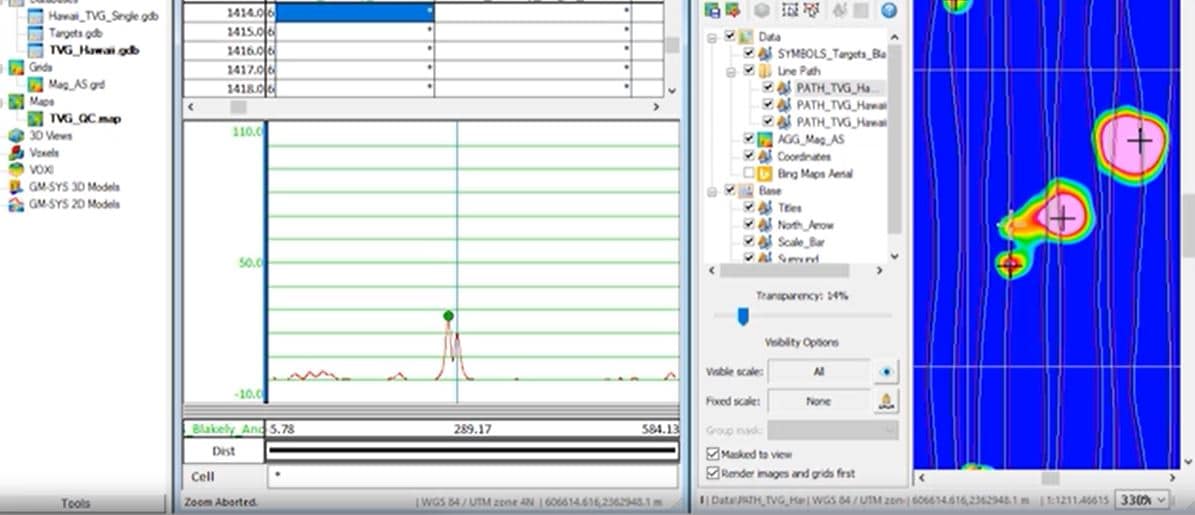
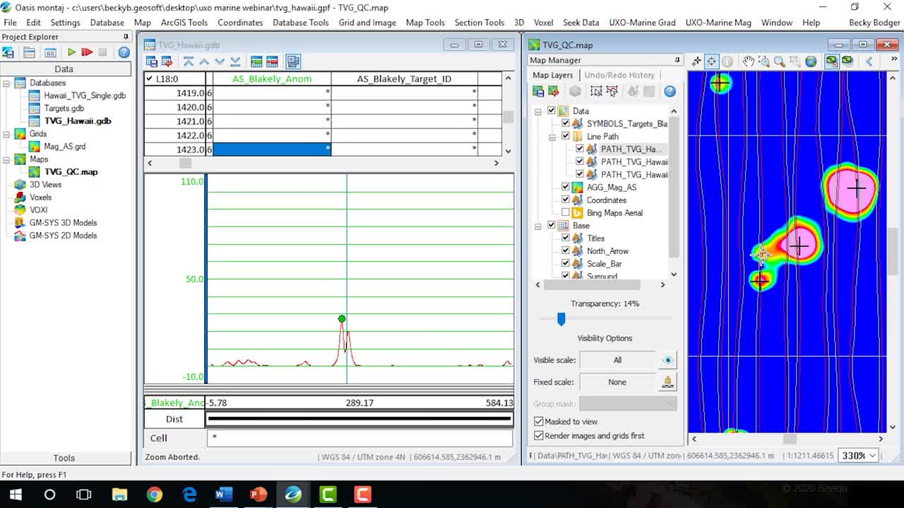
[00:12:48.580]So we have two new channels in our survey database,

[00:12:51.920]we have analytic signal Blakely group anomaly,

[00:12:56.100]and we have the analytic signal Blakely target ID.

[00:13:02.910]So let’s just clean up our database shortcut,

[00:13:06.980]if you’re not aware of getting rid of your profiles

[00:13:08.920]really quickly is to click on one of the numbers

[00:13:12.670]in the y-axis and just press delete.

[00:13:15.210]That just sort of clears it away.

[00:13:18.750]Now I want to display the anomaly value,

[00:13:21.370]however, I don’t have an analytic signal channel

[00:13:24.600]in my survey database,

[00:13:26.100]and that’s because we calculated

[00:13:27.880]the analytic signal from grids.

[00:13:30.460]So the first thing I can do

[00:13:31.960]in order to QCs a position of my target

[00:13:35.930]in the survey database

[00:13:37.610]is to sample the analytic signal grid

[00:13:40.360]back into this database.

[00:13:42.430]I’m going to go to grid and image utilities, sample of grid,

[00:13:49.250]and we’re going to sample the analytic signal grid,

[00:13:52.140]and it’s going to create a new column called AS.

[00:13:59.120]Okay, so now I’m going to display the analytic signal channel

[00:14:04.130]as a profile.

[00:14:06.400]And I’m going to display this analytic signal anomaly

[00:14:11.140]as symbols, so it looks like this channel is empty.

[00:14:16.330]However, if we look at a line

[00:14:21.400]where there’s a potential target, here we go,

[00:14:23.250]we see that there are actually some values in this column.

[00:14:32.580]And I’m going to take,

[00:14:36.290]I’m going to just change my view a little bit,

[00:14:38.100]so I’m going to do statistics of this channel.

[00:14:41.280]So I see that our values are 10 to 108, which makes sense,

[00:14:46.810]so I’m actually going to make this minus 10,

[00:14:50.050]make this 110 and that just brings the zero into our view.

[00:14:57.540]And I’ll be able to see all of the anomalies

[00:15:01.958]in this setup.

[00:15:05.070]So I want to change my y-axis.

[00:15:07.410]I want to make sure that the same axis scale for all lines,

[00:15:11.700]so that when I change lines, my scale doesn’t change.

[00:15:15.450]And again, make sure that the same axis scale

[00:15:17.650]for all profiles is being used.

[00:15:21.650]Okay, so now when I change,

[00:15:23.100]I can see where my anomalies or my targets are.

[00:15:29.230]The other thing I like to do is set up some grid lines.

[00:15:32.760]So if you go to profile option grid,

[00:15:38.130]select display, horizontal grid lines,

[00:15:41.260]and then you can set them up at 10 meter intervals.

[00:15:45.060]And this is really nice

[00:15:46.210]because I can see that this second line here,

[00:15:48.460]so this is the zero line,

[00:15:49.830]and this is my minimum threshold here, my 10.

[00:15:53.860]So anything above that 10

[00:15:55.960]should really have been picked as a target.

[00:16:01.730]However, you will find some that aren’t picked.

[00:16:05.750]And so this is where I’m actually going to verify

[00:16:10.800]with my map, why it wasn’t pick,

[00:16:17.410]so I’m turning everything off

[00:16:18.740]except the analytics signal and the symbols.

[00:16:25.060]And I’m going to zoom in.

[00:16:32.760]And this is where the data linking comes into play.

[00:16:35.050]So we’ve always had this tool here, this data linking tool,

[00:16:39.980]you click it,

[00:16:41.254]and then you can select one of the vectors

[00:16:43.750]that are displayed on your map.

[00:16:45.290]That link back to the database

[00:16:46.900]you’re trying to build the connection to.

[00:16:50.020]So since I’m linking it to the TVG Hawaii database,

[00:16:53.570]I need to select one of these three.

[00:16:55.870]So I’m just going to select the central line path

[00:17:00.800]that I have displayed here.

[00:17:03.340]And it actually doesn’t have to be displayed,

[00:17:05.670]currently displayed,

[00:17:06.620]as long as it shows up in the map manager.

[00:17:10.860]This tool has been around for a long time.

[00:17:13.170]And basically if I click on the map,

[00:17:15.280]it updates the location in the database.

[00:17:17.540]What it never really did effectively was you can see how,

[00:17:22.380]as soon as my cursor goes out of you,

[00:17:24.800]it didn’t change the position of my map,

[00:17:27.720]so it didn’t really track the cursor very well.

[00:17:32.330]So what we added for UXO is this button in the database,

[00:17:35.900]which is called panda cursor on all maps,

[00:17:38.640]it basically tracks your cursor on the map.

[00:17:41.970]You can click in the map and this time now you’ll see

[00:17:44.670]that your map is updating with the position,

[00:17:49.580]which means I can start looking through my database again.

[00:17:54.670]And I can look for some of these anomalies

[00:17:58.560]that are above the 10, the minimum threshold,

[00:18:03.850]but are not selected.

[00:18:05.730]So let’s just look at this one,

[00:18:08.660]so this is basically part of a larger anomaly.

[00:18:16.670]Picking up where we left off in the previous section,

[00:18:19.490]let’s look at adding additional targets

[00:18:21.410]from your survey database.

[00:18:24.610]So going back into Oasis montaj,

[00:18:26.750]I’ve zoomed in here on one of those targets

[00:18:31.010]where we can see from the survey database here

[00:18:36.930]that we have what looks like an anomaly,

[00:18:42.280]but it didn’t get picked,

[00:18:43.620]so it’s above the minimum threshold.

[00:18:47.320]It’s part of it is part of a larger anomaly, and actually,

[00:18:53.010]but it’s far enough away that it has potential

[00:18:55.940]of being some separate UXO so like,

[00:19:01.820]what if this is one of those examples

[00:19:03.450]where we had two very close together.

[00:19:07.980]If we had actually lowered our picking parameters,

[00:19:12.550]so for example,

[00:19:13.383]if we go back and look at the Blakely method,

[00:19:17.290]and this level of peak detection,

[00:19:19.620]if we had lowered it to even more peaks,

[00:19:22.860]which basically is equivalent of two directions,

[00:19:26.380]so it has to find a discreet peak

[00:19:30.080]in only two of the four directions.

[00:19:32.990]So we chose our targets

[00:19:35.620]using the normal peak detection level,

[00:19:38.260]which means four directions,

[00:19:40.580]but I’ve tested this anomaly specifically,

[00:19:42.750]and that it would get selected

[00:19:44.770]as a separate anomaly if we lowered it.

[00:19:49.210]So you have a couple of choices,

[00:19:50.740]like if you start to see a lot of anomalies

[00:19:52.810]that look like that, and you really want them to be picked,

[00:19:55.260]you can rerun your picking algorithm

[00:19:57.220]and select even more peaks to get more targets selected.

[00:20:02.160]But if you only see one or two here and there,

[00:20:03.910]there’s not really a need to rerun and add way more,

[00:20:10.090]then you really see that’s really necessary.

[00:20:13.030]What I can do instead is I can just add

[00:20:16.640]one or two extra targets from manual inspection.

[00:20:21.630]So to do that, we’re going to use the right click menu

[00:20:27.540]from the profile window.

[00:20:29.270]So when you right click,

[00:20:30.620]and if you have your UXO Marine menus loaded,

[00:20:33.990]you’ll notice that you have a whole bunch of new menu items

[00:20:38.200]in the right click menu.

[00:20:40.570]And then one we’re going to use is the Marine mag ones,

[00:20:43.170]so the first thing is click on settings,

[00:20:46.060]so UXO Marine mag add/remove target settings.

[00:20:49.590]And this looks a little bit like our target picking,

[00:20:53.460]the Blakely method, and it’s basically the same,

[00:20:56.750]so this is just telling it where to save the targets

[00:20:59.660]that we are going to manually select.

[00:21:02.490]So we just set it up like we did the previous step,

[00:21:05.510]so the survey database is the TVG Hawaii.

[00:21:09.120]The channel to pick anomaly from his analytics signal.

[00:21:12.480]Our base level is zero,

[00:21:13.820]since we did a pretty good background removal.

[00:21:18.010]If you’re picking from TMI or a total field,

[00:21:23.085]you could select negative peaks as well as positive peaks.

[00:21:26.820]I really like this option,

[00:21:28.310]which is snapped to the closest peak,

[00:21:30.420]and that means I don’t have to click

[00:21:32.330]the exact highest peak of the target,

[00:21:36.900]it will find it for me automatically.

[00:21:40.120]This is one example

[00:21:41.270]where you can bring over additional data,

[00:21:44.300]but since we didn’t do it with the Blakely picking,

[00:21:46.360]we’re not going to do it here,

[00:21:47.310]we’re going to actually look at that at this

[00:21:48.840]as the next step.

[00:21:51.280]And we’re going to tell it to pick from,

[00:21:56.360]we’re going to save it to the target,

[00:21:57.890]to the same Blakely group and that’s it.

[00:22:01.000]Click, okay.

[00:22:02.030]Now that doesn’t actually do anything,

[00:22:03.210]that’s just setting it up.

[00:22:06.727]So the next step

[00:22:07.560]is to actually select the target you want to add.

[00:22:11.620]And again, you don’t have to find the highest peak,

[00:22:13.750]you can just click somewhere near it,

[00:22:15.580]and then you’re going to right click,

[00:22:16.730]and you’re going to click add target.

[00:22:20.780]And because we set it up

[00:22:23.580]to save to the exact same target list,

[00:22:26.210]it’s going to add it to the same channel

[00:22:28.550]in the survey database,

[00:22:31.080]but it does not add the symbol to our map

[00:22:33.780]that we can add manually.

[00:22:35.350]So if we just go to map tools, symbols, location plot,

[00:22:41.360]we’re going to use the plus sign,

[00:22:42.900]we’re going to pick us a mask channel.

[00:22:45.620]We don’t want every row to show up,

[00:22:51.040]so we don’t want the line path defined,

[00:22:53.470]we just want the AS Blakely anom channel.

[00:22:58.810]So that’s somewhere in here.

[00:23:06.630]AS Blakely anom is the very last one in the database,

[00:23:09.920]of course.

[00:23:12.110]Click, okay.

[00:23:12.943]And you see, so now it’s added,

[00:23:15.570]we can remove the previous one actually,

[00:23:17.300]and it’s added the new one

[00:23:19.460]that we’ve just selected from our database.

[00:23:24.830]For this next section,

[00:23:25.800]we’re going to look at the importance of target size

[00:23:28.350]when modeling depths.

[00:23:30.590]So both euler deconvolution and batch fit modeling methods

[00:23:37.100]work inside a target window.

[00:23:39.520]The window is based on your target size

[00:23:42.380]and it defines what points are used

[00:23:45.280]during the modeling process.

[00:23:47.730]The goal of your window or target size

[00:23:49.760]should be as big as possible over a single anomaly.

[00:23:55.300]We’re going to change gears

[00:23:56.220]and look at a vertical gradient survey.

[00:23:59.870]This has actual UXOs and the size of the window,

[00:24:03.953]and the size of the targets that we’re looking at

[00:24:06.640]are a bit smaller than the Hawaiian dataset,

[00:24:10.580]so I think this is a better example.

[00:24:14.560]We have a map with the analytics signal displayed,

[00:24:18.810]I have my survey database, and I have a target list here.

[00:24:22.620]Now, admittedly, I’ve shortened it,

[00:24:24.120]I’ve picked just six targets to focus on,

[00:24:26.940]so let’s zoom in on our map.

[00:24:30.080]Let’s just zoom into the middle portion here.

[00:24:32.290]And then we’re going to use the data linking

[00:24:34.870]to really find and look at where our targets lie.

[00:24:46.740]Okay, so you can see I’ve selected a couple

[00:24:50.480]that are close together, some that are far apart,

[00:24:54.700]and big and small.

[00:24:59.480]So as I mentioned before,

[00:25:00.930]the real goal when you’re modeling your target

[00:25:03.540]is to pick the correct window size.

[00:25:05.870]This is one of the biggest influencing factors

[00:25:08.490]of getting good model of depth.

[00:25:11.650]So we’re going to go to UXO Marine mag

[00:25:14.020]calculate anomaly sizes.

[00:25:16.690]This uses the analytic signal

[00:25:18.630]to define the footprint of your anomaly.

[00:25:22.800]So our target database

[00:25:23.850]is this targets for modeling Blakely group,

[00:25:27.670]and we’re going to output the size to a size channel.

[00:25:35.120]Okay, so one thing to note for euler deconvolution,

[00:25:40.510]the size that’s listed in the size channel is only a radius,

[00:25:43.950]it’s a half width.

[00:25:45.890]So if we want to visualize what the window is,

[00:25:49.330]that is based on this size,

[00:25:52.410]we need to actually create a box around the anomaly

[00:25:57.160]that’s twice the size listed here.

[00:26:00.320]So to do that,

[00:26:01.153]we’re going to use something called proportional symbols.

[00:26:03.600]In order to use proportional symbols on the map,

[00:26:06.480]we need to know what the scale of this map is.

[00:26:09.020]So one of the ways that you can just double check

[00:26:11.840]is to go to map tools, base map, draw base map,

[00:26:16.440]and we’re not actually going to redraw our base map,

[00:26:18.480]we’re just looking at the scale that’s set here.

[00:26:21.440]So this is at one to 25,000, so I’m just going to cancel that.

[00:26:25.360]Okay, now let’s go to map tools, symbols, proportional size.

[00:26:34.000]The data channel that we want to use is the size channel,

[00:26:36.820]zero-based level is zero, and the scale factors,

[00:26:40.320]so this is one to 25,000.

[00:26:42.840]If we wanted to draw a box,

[00:26:44.210]that was exactly the size listed here,

[00:26:46.490]we would just divide that 25,000 by 1,000,

[00:26:49.790]which would make it 25.

[00:26:51.740]But because we’re trying to double the size listed here,

[00:26:55.330]we’re going to cut it in half again.

[00:26:57.200]So it’s going to be 25,000 divided by 1,000, divided by two,

[00:27:02.050]and that gives us 12.5.

[00:27:04.640]The symbol I like to use is this box one,

[00:27:07.550]and I set the edges to be ultra light,

[00:27:11.800]so I don’t get a thick line. I get a thin line.

[00:27:14.500]Click, okay.

[00:27:15.750]Click, Okay, again.

[00:27:18.290]And it will draw some squares over our anomalies.

[00:27:23.840]Okay.

[00:27:26.538](Becky clears throat)

[00:27:27.700]So if we look at each of these windows,

[00:27:30.810]the first thing you should notice is that in general,

[00:27:33.170]they’re too small.

[00:27:35.830]So there’s a couple of things you can do.

[00:27:37.127]One of the first things lots of people do

[00:27:38.930]is just multiply this size by two.

[00:27:42.340]So we can use channel math to do that.

[00:27:47.040]We’re going to do a simple C0 = C1 times two,

[00:27:53.120]and this C0 will be called size_double,

[00:28:00.296]something like that.

[00:28:01.220](Becky chuckles)

[00:28:02.053]And we’re going to select the size channel

[00:28:03.910]and click apply, no errors, so I’m going to click close.

[00:28:09.940]And now we have twice that size,

[00:28:12.640]and this time we’re going to plot the size double.

[00:28:26.790]Okay and as we look now,

[00:28:30.430]we can see that they’re actually a little bit better,

[00:28:39.530]but there’s still a few issues, okay.

[00:28:45.570]So we’re going to use this size double channel,

[00:28:47.620]and we’re going to just refine this a little bit.

[00:28:49.460]So this last one, this one here,

[00:28:51.560]we can make this even bigger.

[00:28:53.100]So remember the point here is to make it as big as possible

[00:28:56.740]without touching another anomaly basically,

[00:28:58.980]’cause we only want the data for one anomaly

[00:29:01.730]included inside this window.

[00:29:03.500]So I’m actually going to just manually type 15 in that cell

[00:29:07.990]and see what happens.

[00:29:15.620]So that’s looking a bit better.

[00:29:16.790]I can go even bigger, maybe 20.

[00:29:31.250]And that’s looking better.

[00:29:33.520]So you don’t the problem with these narrow surveys

[00:29:38.050]is that you also can’t have too many dummies

[00:29:40.570]inside your window.

[00:29:41.890]This should be okay, but if at some point,

[00:29:45.550]if it reaches too many dummies, you won’t find a solution,

[00:29:50.750]so you have to be careful of that as well.

[00:29:53.470]So let’s move on.

[00:29:54.630]So let’s look at these two anomalies.

[00:29:56.560]Let’s turn off the first ones

[00:30:01.665]and let’s just look at the double sized ones.

[00:30:04.740]So, (Becky clears throat)

[00:30:06.490]when they’re really close together, we have another problem.

[00:30:09.520]And that is that we have to make it as big as possible,

[00:30:11.670]but we can’t include much from the other anomaly.

[00:30:16.550]So for the first one, I think the size is just right.

[00:30:24.070]It’s touching it a little bit in the corner here,

[00:30:26.120]but if we go as much smaller,

[00:30:27.490]we’re going to leave out some of the crucial information,

[00:30:30.490]so I’m going to leave that one alone.

[00:30:34.810]But this one here,

[00:30:35.700]you can see that it’s picking up a large part

[00:30:37.970]of its neighboring anomaly,

[00:30:40.910]so we’re going to reduce the size of this one.

[00:30:43.200]We’re going to make it six, and then let’s redraw the symbols,

[00:30:49.680]and see what happens to it.

[00:30:55.840]That’s better.

[00:30:58.310]Maybe we could go a little bit bigger.

[00:31:08.960]Yeah, so we’re still picking up a little bit

[00:31:10.320]in the corner here,

[00:31:11.430]but the most important thing I think is that

[00:31:13.910]we’re also picking up the entirety of the large portion

[00:31:19.590]of the actual anomaly.

[00:31:21.750]Now the boxes can overlap.

[00:31:23.310]That has no impact on the modeling

[00:31:28.150]because they’re treated one at a time.

[00:31:32.042]Okay, so let’s move on to the next one.

[00:31:34.520]This one is set to 4.9,

[00:31:36.130]but I think actually can go a lot bigger.

[00:31:38.100]I think, let’s try doubling it,

[00:31:40.690]more than doubling it in that case.

[00:31:43.290]Let’s adjust this one.

[00:31:45.300]This one looks a bit big,

[00:31:47.440]so let’s try setting it to maybe eight,

[00:31:50.950]and this one I’m going to just round it off,

[00:31:55.020]bring it down to seven.

[00:31:57.910]And let’s display the symbols again

[00:32:00.370]and just see what happened when we change those.

[00:32:08.620]Okay, so that didn’t really make much of a difference,

[00:32:10.910]but that’s fine, we’ll just leave it.

[00:32:12.510]And then this is the eight,

[00:32:15.310]that’s fine, let’s leave that one also.

[00:32:18.260]And this is 10, so I think this is big enough.

[00:32:20.560]Again, it has some dummies in the corner,

[00:32:22.280]but I don’t think there’s too many there,

[00:32:23.610]so I think that that will run just fine.

[00:32:27.740]All right.

[00:32:30.210]So once we’re happy with that size,

[00:32:32.100]we can actually run the tool

[00:32:34.010]and let’s see what it gives us for a depth.

[00:32:38.800]So I’ve run through this once already,

[00:32:40.300]so the defaults are still saved.

[00:32:43.020]So it’s going to look for our target database.

[00:32:45.620]The group is called, Blakely.

[00:32:47.872]We’re going to start with a three ordinance.

[00:32:51.030]There’s a really good webinar by Alan Reed,

[00:32:54.360]and he talks a lot about the different structural index

[00:32:58.900]when you’re running euler,

[00:32:59.780]and I highly recommend watching that.

[00:33:01.640]I can link to it at the end, if you like.

[00:33:04.630]It’s picking up the target size channel,

[00:33:07.660]which is our double one.

[00:33:09.250]And we’re going to put in the instrument height,

[00:33:11.100]which is 2.5.

[00:33:12.610]And then we’ve already calculated all of these grids.

[00:33:15.350]So it knows what our analytics signal crit is,

[00:33:18.170]our total field, and then our gradients in each direction,

[00:33:21.370]which were derived, in this case,

[00:33:22.850]from the vertical derivative.

[00:33:25.970]So let’s click okay, and let it run.

[00:33:30.330]And there we have it.

[00:33:31.163]So now we have a depth, a weight, and an air channel.

[00:33:36.380]This is a percentage, so those are all really low,

[00:33:38.290]so that’s, I say those are all acceptable.

[00:33:42.600]Okay, let’s talk about the size now for batch fit modeling.

[00:33:46.770]It also needs a window size,

[00:33:48.790]however, it doesn’t use a size channel, unfortunately.

[00:33:52.740]Instead, what it needs,

[00:33:54.520]if we look at the dialogue here

[00:33:55.810]is we have to specify a window size and we can only run,

[00:34:00.560]we can only model on one window size at a time.

[00:34:03.780]So what we’re going to do,

[00:34:04.613]is we’re going to use the mask channels.

[00:34:06.000]And what we’re going to do is we’re going to create

[00:34:07.670]separate mask channels for each group of sizes,

[00:34:10.857]and we’re going to populate it,

[00:34:12.380]and then we’re going to run through batch fit,

[00:34:15.780]as many times as we have different sized windows.

[00:34:19.410]We can’t run it all at one size

[00:34:21.610]because you saw from the previous step,

[00:34:23.470]how they vary so much.

[00:34:25.750]And just like euler,

[00:34:27.400]the window size is one of the most impactful settings

[00:34:31.990]that will give you good results.

[00:34:33.910]So let’s just cancel this and come back to our database.

[00:34:38.170]I’m going to move this size double.

[00:34:41.410]I’m going to hide the column and display it at the end.

[00:34:48.080]Okay, and the first thing we want to do with this

[00:34:54.540]is actually reduce the number of different sizes

[00:34:56.940]that we have,

[00:34:57.773]so we can do this by sort of bucketing the size.

[00:35:02.360]If we look at these two, for example,

[00:35:08.270]now I’m using a window size of seven

[00:35:10.240]for the one in the bottom right-hand corner

[00:35:11.620]and eight up here.

[00:35:12.940]But actually I could probably increase

[00:35:15.230]this one at the bottom a little bit bigger,

[00:35:17.330]make it a bit bigger.

[00:35:18.170]So if I set that one to eight,

[00:35:20.890]the amount of times

[00:35:21.900]that we actually have to run through batch fit

[00:35:23.840]is now reduced by one, right?

[00:35:25.710]Because now I can run both of these targets

[00:35:29.150]at the same target size,

[00:35:32.146]redisplay our symbol, proportional sizes,

[00:35:34.680]if we want to see what that looks like.

[00:35:37.160]And see that it gets a little bit bigger, but that’s okay,

[00:35:44.390]and I think it’ll still give us good results.

[00:35:47.270]This one is set to 10 that’s we’re going to leave that one.

[00:35:51.180]And then these two here, maybe, actually we can,

[00:35:57.240]maybe they both look okay at six.

[00:36:01.560]So let’s run the proportional symbol one more time.

[00:36:12.780]So now instead of running it,

[00:36:14.760]running batch fit six times with six different sizes,

[00:36:17.240]we’re actually just going to run it four times.

[00:36:20.550]So the next step that we have to do,

[00:36:21.770]is we have to create our mask channels.

[00:36:24.060]So we’re going to create a mask eight.

[00:36:28.980]And we have to actually set the class here as mask.

[00:36:34.040]And we’re going to just populate it with a one

[00:36:35.970]for each of the sizes that are eight.

[00:36:39.840]And then we’re going to do the same with mask 10,

[00:36:44.466](keyboard typing)

[00:36:49.130]mask six,

[00:36:53.518](keyboard typing)

[00:36:57.340]and mask 20.

[00:37:04.089](keyboard typing)

[00:37:08.300]Okay, and then we’re going to put a one

[00:37:12.150]wherever it matches the size.

[00:37:17.210]There’s a way to easily populate these ’cause again,

[00:37:19.680]I’m very much aware

[00:37:20.750]that when you’re doing this with a real survey,

[00:37:22.540]you’re going to have hundreds of targets,

[00:37:25.090]so this is a time consuming process.

[00:37:27.660]You can use channel math,

[00:37:30.070]if you use a true false statement.

[00:37:33.750]Just going to clear this and we’re going to load

[00:37:35.830]the true false statement from common tasks.

[00:37:38.270]What you can say is where C0 equals a specific value,

[00:37:43.110]like eight, then put a one in the resulting channel.

[00:37:48.410]Otherwise, leave it as a dummy.

[00:37:50.990]And so what you say for C0

[00:37:53.580]this will be set one of your mask channels, so eight,

[00:37:56.930]and this will be sized double.

[00:37:58.430]And so what we’re seeing with this is,

[00:38:00.220]everywhere there is, everywhere size double equals eight,

[00:38:04.190]it’s going to put a one, otherwise, dummy it.

[00:38:09.420]You can script this.

[00:38:11.210]So if you just have a list of the sizes that you’ve used,

[00:38:13.650]and if you’ve bucketed them into round even numbers,

[00:38:16.530]then it shouldn’t be too difficult

[00:38:17.870]and you can automate this task.

[00:38:21.050]And yeah, so once we have our mask channels like this,

[00:38:24.660]we can actually run through the batch fit process.

[00:38:28.840]So we have our targets for modeling database.

[00:38:33.120]We’re going to start with mask eight.

[00:38:37.500]If we want to use the actual altitude channel

[00:38:41.400]from our survey database, we can,

[00:38:44.860]or we can use the instrument height above ground.

[00:38:46.650]So we’re going to just run it just like we did for euler,

[00:38:49.040]so I’m going to use the instrument height above the ground.

[00:38:51.890]So our mag channel in the survey database is the residual,

[00:38:55.710]our target window size, so this is the next part that might,

[00:38:59.950]you might get wrong if you’re not aware of it.

[00:39:03.210]Remember that I mentioned before that for Euler,

[00:39:06.320]this size is a radius, so it’s a half width.

[00:39:09.790]But for batch fit is asking you for the full window size,

[00:39:13.950]so we’re actually going to double the size

[00:39:16.330]that we specified here.

[00:39:17.540]So if this is mask eight, we’re actually going to put in 16.

[00:39:21.840]Okay, and I think the survey was maybe from 2016,

[00:39:28.700]I don’t have the exact date,

[00:39:30.800]but we’ll just put January, 2016,

[00:39:34.060]and make sure that you calculate that correct,

[00:39:37.610]getting the IGF parameters that’s used for batch fit.

[00:39:40.980]And it creates polygons of your target window,

[00:39:47.300]the modeling window that it’s using,

[00:39:48.940]and we’re going to look at those afterwards

[00:39:50.450]to verify that we got the right size.

[00:39:53.350]All right, so let’s click, okay.

[00:39:56.030]And it’s saying that my directory

[00:39:58.650]for saving those polygons doesn’t exist,

[00:40:00.380]do I want to create it?

[00:40:01.213]Yes.

[00:40:03.680]And then let’s let it run, it shouldn’t,

[00:40:05.260]again, it shouldn’t take very long,

[00:40:06.390]it’s only modeling two targets.

[00:40:08.820]This is another part though,

[00:40:10.130]where we get a lot of questions in support.

[00:40:12.960]Batch fit modeling is very computationally heavy.

[00:40:15.780]You can see how long it’s taking just for two models,

[00:40:18.480]for two target, sorry.

[00:40:21.510]And so sometimes you will not be able to run

[00:40:24.600]an entire target list in one go, you’ll have to split it up.

[00:40:29.470]But if you’re bucketing,

[00:40:30.577]and you’re splitting it up with mask channels, that’ll help.

[00:40:34.340]But I wouldn’t necessarily recommend running 500 targets

[00:40:38.070]at once through batch fit.

[00:40:42.440]Okay, so we have a result.

[00:40:43.880]And if I scroll down to the end,

[00:40:46.710]we have all these fit, new fit channels.

[00:40:49.160]So anything with fit in the name

[00:40:51.290]is a result from the batch fit modeling.

[00:40:54.150]So we have the new X and Y position

[00:40:55.960]of our target depth below sensor, size,

[00:41:00.230]coherence which is how well the data fit the model,

[00:41:04.100]error, inclination,

[00:41:05.440]declination of our dipole magnetic moment

[00:41:07.650]and an angle between the Earth’s magnetic field.

[00:41:11.470]So the last thing I want to,

[00:41:16.130]I’m not actually going to run through

[00:41:17.610]the rest of the targets as you go through batch fit

[00:41:23.230]and change the mask channel and window size,

[00:41:27.010]it just fills in the blanks

[00:41:29.100]that are left behind in this database.

[00:41:32.340]So the last part was target size, and I promise this is it.

[00:41:37.010]The first time you do this,

[00:41:38.150]you’ll probably want to verify

[00:41:39.130]that you got the polygons right for the batch fit.

[00:41:42.540]So we can go to our map

[00:41:43.720]and we can actually display the polygon

[00:41:47.200]that was created during batch fit,

[00:41:49.210]so we’re going to draw from PLY file.

[00:41:52.780]You’re going to click browse,

[00:41:53.900]and inside your working directory

[00:41:55.640]is a folder called work and then PLY,

[00:41:59.779]and we’re going to select one of these polygons.

[00:42:03.660]Make sure that your line thickness isn’t too big,

[00:42:05.790]and then click, okay.

[00:42:07.520]And it’s actually going to just draw the symbol

[00:42:09.610]and you can see now it’s matched our proportional symbols

[00:42:14.530]that we created from our size double channel exactly,

[00:42:19.330]so I’m confident that we used the right window size

[00:42:22.840]and that’s just a nice little verification,

[00:42:25.190]if you’re unsure,

[00:42:26.290]if you can’t remember the rules about when it’s a radius

[00:42:29.060]or when it’s the full window width.

[00:42:33.460]The next tip we’re going to look at

[00:42:34.600]is updating your target list with additional data.

[00:42:38.380]The results from our depth modeling,

[00:42:41.710]we have two depth channels now.

[00:42:43.430]We have a fit depth from batch fit,

[00:42:46.240]and we have our mag depth which is from euler.

[00:42:53.890]Both of these results are depth below the sensor,

[00:43:00.010]So, (indistinct) is bring in our altitude channel,

[00:43:04.700]subtract the altitude from both these depths,

[00:43:08.250]and that will give us a depth below seabed.

[00:43:13.260]So to do that,

[00:43:14.093]we have a nice tool under managed targets,

[00:43:18.440]called update target list,

[00:43:20.210]and this is basically just a cross channel lookup.

[00:43:23.860]So you give it your survey database, the vertical gradient,

[00:43:27.170]we’re going to give it the target ID channel.

[00:43:29.470]Now this target ID channel exists

[00:43:32.020]in both the survey database and our target database.

[00:43:35.670]And this is the channel it’s going to use as a reference

[00:43:38.670]to bring across the additional values, the additional data,

[00:43:45.930]so this is the AS Blakely target ID.

[00:43:49.690]This is where we can select those additional channels,

[00:43:51.810]so I want to bring across my despiked

[00:43:55.740]and smoothed altitude channel.

[00:43:58.260]And if there’s anything else you wanted to bring across,

[00:44:03.600]for example, if you wanted to look at your background,

[00:44:05.810]or if you want your depths or time

[00:44:08.990]or anything else that you might have in your survey,

[00:44:11.450]we’re just going to bring the one across for now.

[00:44:13.610]And then in your target database,

[00:44:14.990]make sure that you set the same,

[00:44:17.360]so it’s target for modeling Blakely group mask channel,

[00:44:21.090]that’s fine.

[00:44:22.160]So we click, okay.

[00:44:23.370]And now you can see that we actually have our altitude

[00:44:26.230]at each of the target locations.

[00:44:31.330]The final step would be to use channel math

[00:44:33.170]to calculate the depth below seabed.

[00:44:35.760]So we’re going to clear that,

[00:44:37.160]and we’re going to do another simple expression,

[00:44:39.460]which is C1 minus C2, C0 we could call it,

[00:44:45.860]we’ll use the same naming convention,

[00:44:47.920]so we’ll call it fits_depth_BSB for below seabed,

[00:44:56.150]and C1 is our fit depth, and C2 is the altitude.

[00:45:06.420]I’m going to click apply, and that gave me the first channel.

[00:45:10.750]And then we’re going to just change this, so the new one,

[00:45:14.720]for the second one we’re just going to call it, mag_depth,

[00:45:20.600]and C1 is mag_depth, and altitude stays the same.

[00:45:32.410]And there we have a depth from batch fit,

[00:45:37.160]and a depth from euler,

[00:45:40.130]and you can see that they’re pretty similar,

[00:45:42.160]so I’m happy with those results.

[00:45:45.340]The last step that we’re going to look at today,

[00:45:46.940]is survey coverage.

[00:45:48.100]And this is going to be more of a demonstration

[00:45:50.060]of how the tool works.

[00:45:54.320]So we’re going to calculate the percentage of coverage

[00:45:58.710]that they had within this red polygon on my map here,

[00:46:02.360]for the vertical gradients survey.

[00:46:05.060]Now there’s a couple of things that you need to know

[00:46:07.970]before you run the tool.

[00:46:10.270]The first thing is you have to have this boundary outline,

[00:46:14.290]and it’s usually delivered to you by the customer

[00:46:16.190]because it’s the area that they want you to survey within.

[00:46:20.730]And it can be a shape,

[00:46:21.750]it can sometimes be delivered as a shape file,

[00:46:23.990]it could be a polygon file,

[00:46:25.140]or can even just be a set of coordinates

[00:46:27.130]of the corner locations or something like that.

[00:46:30.580]I’ve saved it as a polygon file and I’ve displayed it here,

[00:46:33.360]so if we just zoom in, we can see it’s just an outline.

[00:46:37.500]See that even with the gradient that we have some gaps,

[00:46:39.720]so I’m not expecting 100% coverage

[00:46:41.840]within this survey boundary.

[00:46:44.950]The other thing that you need to know

[00:46:46.210]is the maximum detection range.

[00:46:49.160]And so this is going to be different for every survey

[00:46:53.720]based on the type of UXO you’re looking for,

[00:46:55.810]and also the depth below the seabed that you have to clear.

[00:46:59.580]So for this survey, we’re going to use eight meters.

[00:47:02.970]And if they’re 2.5 meters above the surface,

[00:47:08.250]they can clear up to a 5.5 meters below the surface.

[00:47:12.920]And the last thing is that you can’t have any dummies

[00:47:15.810]in your altitude channel,

[00:47:17.080]so this is a dynamic survey coverage tool.

[00:47:19.910]So it looks at the altitude at that you’re you’re at

[00:47:23.290]as part of the calculation.

[00:47:26.033]And so, yeah, just one of the tips here,

[00:47:27.210]is that you can’t have any dummy in your altitude channel.

[00:47:31.330]So let’s look at the tool.

[00:47:32.700]So if we go to survey coverage,

[00:47:35.260]we’re going to run it on our vertical gradient database,

[00:47:37.810]that’s our survey database.

[00:47:39.270]We’re going to tell it what the altitude channel is.

[00:47:41.713]We’re going to give it the survey boundary.

[00:47:43.340]If you have an exclusion zone,

[00:47:45.900]like an island or something that you had to go around

[00:47:47.910]within the larger boundary,

[00:47:49.900]you can set that here,

[00:47:50.927]and that will just remove that area

[00:47:52.610]from your percentage calculation.

[00:47:55.460]The footprint shape we’re going to use

[00:47:57.190]is a circle that works best for magnetic surveys.

[00:48:01.840]If you have a really big area,

[00:48:03.500]you can reduce the resolution of the circle.

[00:48:05.890]And that just means the number of points or like vertices

[00:48:09.770]that are used to define the shape of the circle,

[00:48:12.500]and it can speed up the process a little bit.

[00:48:15.280]The footprint size here is the maximum detection range,

[00:48:17.730]and this is where we’re putting in our eight meters.

[00:48:20.640]And we’re going to display the coverage on our current map,

[00:48:23.080]and we’re going to plot our legend.

[00:48:25.630]So click, okay.

[00:48:27.440]And then we’ll let that run.

[00:48:33.000]So I actually canceled it,

[00:48:34.050]’cause I’ve already run this tool and I don’t want to just,

[00:48:36.050]I don’t want to spend too much time letting it run.

[00:48:38.590]I just want to show you the results of that tool.

[00:48:41.530]Once it completes,

[00:48:43.570]you get this nice calculation

[00:48:45.530]in your legend of the percentage coverage.

[00:48:48.490]So we can see that with a footprint of eight meters,

[00:48:51.290]we have a 98% coverage within the boundary that we selected.

[00:48:55.180]Let’s just zoom in and look at the actual map itself.

[00:48:59.570]And you can see that we get this gray area

[00:49:03.150]and it shows you where the gaps are.

[00:49:05.060]Now, if in your contract,

[00:49:06.800]it says you have to have 99% coverage,

[00:49:09.790]then you might have to come in here

[00:49:11.580]and fill in some of these areas,

[00:49:15.590]but that’s all there is to it really.

[00:49:16.890]So it’s a nice, easy tool to use,

[00:49:19.480]and it gives you a pretty decent map that you can deliver

[00:49:24.100]that shows the coverage that you achieved on your survey.

[00:49:30.200]That’s all the tips I have for today.

[00:49:32.030]To recap, we covered a brief overview

[00:49:33.930]of a typical UXO Marine workflow in Oasis montaj.

[00:49:37.220]We looked at setting up your database

[00:49:38.790]for QC in multiple lines.

[00:49:41.030]Viewing targets in the survey database

[00:49:42.980]and data linking between your target database and maps.

[00:49:45.810]Adding additional targets manually to your target list.

[00:49:49.100]We discussed that length,

[00:49:50.560]the importance of target size for modeling depths

[00:49:53.150]in both euler and batch fit.

[00:49:55.340]Updating your target list with additional data

[00:49:57.330]and survey coverage.