Groundwater Pumping and Drawdown Maps in SEEP3D

The ultimate goal of a dewatering analysis is to understand the transient response of the flow system and determine pumping rates, pore-water pressure distribution, and the extents of drawdown. This webinar demonstrates the creation of two three-dimensional groundwater dewatering problems and their associated drawdown conditions. The results of the SEEP3D analyses are then exported into the third party software, Python, for the creation of drawdown maps.

Overview

Video Transcript

[00:00:01.670]
<v [Instructor>Hello and welcome to this GeoStudio webinar</v>

[00:00:04.610]
that focuses on both de-watering,

[00:00:06.880]
which includes pumping and pressure relief systems,

[00:00:10.121]
and drawdown maps in SEEP3D.

[00:00:14.030]
My name is Marc LeBeau

[00:00:15.440]
and I’m a research and development scientist

[00:00:17.830]
with the Geoslope engineering team at Seequent.

[00:00:21.660]
Today’s webinar will be approximately 30 minutes long.

[00:00:25.910]
Attendees can ask questions using the chat feature

[00:00:29.070]
and I will respond to these questions via email

[00:00:31.900]
as quickly as possible.

[00:00:34.230]
It should be noted that a recording of the webinar

[00:00:37.060]
will be available so participants

[00:00:38.830]
can review the demonstration at a later time.

[00:00:43.940]
Geostudio is a software package developed

[00:00:46.540]
for geotechnical engineers and earth scientist

[00:00:49.480]
which is comprised of several products.

[00:00:52.449]
The range of products allows users

[00:00:54.950]
to solve a wide array of problems

[00:00:56.810]
that may be encountered in these fields.

[00:00:59.390]
Today’s webinar will focus on Seep3D.

[00:01:03.220]
Those looking to learn more about the products,

[00:01:05.720]
including background theory,

[00:01:07.380]
available features and typical modeling scenarios,

[00:01:10.890]
can find an extensive library of resources

[00:01:13.610]
on the Geoslope website.

[00:01:16.330]
Here you can find tutorial videos,

[00:01:19.440]
examples with detailed explanations,

[00:01:22.860]
and engineering books on each product.

[00:01:26.400]
To begin this webinar,

[00:01:27.740]
let’s start by answering three fundamental questions.

[00:01:31.310]
The first question is, why?

[00:01:33.470]
Why should we consider using a de-watering system?

[00:01:37.320]
The second question is, what?

[00:01:40.420]
What are the different types of de-watering systems?

[00:01:43.540]
And the third very important question is, how?

[00:01:48.260]
How can we implement these systems in a numerical model?

[00:01:53.440]
So why exactly should we consider using

[00:01:55.980]
a de-watering system?

[00:01:57.550]
Well, the construction of engineered structures,

[00:02:00.210]
such as buildings, dams, levees and tunnels

[00:02:03.300]
often requires excavation into water bearing soils

[00:02:06.550]
and/or consideration of underlying artesian pressures.

[00:02:10.540]
The reasons for installing a de-watering system

[00:02:13.450]
therefore include, but are not limited to,

[00:02:17.510]
lowering the phreatic surface and intercepting seepage

[00:02:20.620]
that would otherwise emerge from a slope

[00:02:22.760]
or bottom of an excavation,

[00:02:25.550]
increasing slope stability,

[00:02:28.730]
preventing erosion heave and uplift

[00:02:31.290]
that may occur at the bottom of an excavation

[00:02:33.540]
or at the toe of a dam,

[00:02:36.200]
reducing lateral loads on excavation sheeting and bracing,

[00:02:41.510]
and reducing required air pressures

[00:02:43.780]
during tunnel construction.

[00:02:47.750]
There are many types of de-watering systems.

[00:02:50.310]
Some of these systems are quite old

[00:02:52.290]
and were introduced prior to the advent

[00:02:54.540]
of modern well installation techniques

[00:02:57.130]
and pumping apparatus.

[00:02:59.330]
These systems include,

[00:03:02.380]
permanent and less expensive structures,

[00:03:04.690]
such as sumps and ditches that are well adapted

[00:03:07.940]
to small excavations or fine grain soils,

[00:03:14.210]
sheeting and open pumping,

[00:03:18.510]
sheeting with deep-well sumps,

[00:03:20.830]
which are now mostly replaced by wells with screens,

[00:03:24.510]
and more recent techniques,

[00:03:26.160]
which include well point systems in which small wells

[00:03:30.900]
are connected to centrifugal pumps,

[00:03:36.010]
deep well systems in which large diameter wells

[00:03:39.110]
are connected to the submersible or turbine pumps,

[00:03:43.780]
pressure relief systems in which well points

[00:03:46.370]
or deep wells are used to decrease artesian pressures,

[00:03:52.620]
horizontal systems in which horizontal pipes

[00:03:55.590]
are projected from shafts or wells,

[00:04:00.270]
vacuum de-watering systems for fine grain soils

[00:04:03.670]
in which well points are connected to vacuum pumps,

[00:04:07.830]
and finally, electrical systems for very fine grain soils

[00:04:12.580]
in which well points are combined

[00:04:14.330]
with the flow of electricity.

[00:04:18.520]
The first recorded lowering of the phreatic surface

[00:04:21.170]
was achieved in 1838 during the construction

[00:04:24.470]
of the Kilsby tunnel in the United Kingdom.

[00:04:28.320]
In this case, the phreatic surface was lowered

[00:04:30.710]
by pumping from large vertical shafts

[00:04:33.069]
adjacent to the tunnel.

[00:04:38.210]
One of the earliest examples of the use of deep wells

[00:04:41.230]
for pressure relief purposes dates back

[00:04:43.770]
to the construction of the Bremerhaven lock

[00:04:46.900]
or Nordshleuse in 1927.

[00:04:51.410]
The system consisted of 58 deep wells located outside

[00:04:56.200]
of the sheet piling

[00:04:57.600]
and resulted in a 50 foot decrease in artesian pressure.

[00:05:02.783]
Another early example of de-watering is the system used

[00:05:06.680]
for the construction of the Rutgers tunnels

[00:05:09.200]
in New York city.

[00:05:11.530]
The system consisted of five 100-foot deep wells

[00:05:15.380]
equipped with electrically powered deep-well turbine pumps.

[00:05:19.690]
The system allowed for the construction

[00:05:21.600]
of a large portion of the tunnels under free air

[00:05:25.540]
and significantly lowered the air pressure required

[00:05:28.280]
for tunneling purposes.

[00:05:33.940]
The remainder of this webinar will focus on answering

[00:05:37.040]
the “how” question.

[00:05:38.430]
And this will be done by modeling two de-watering systems.

[00:05:42.600]
The first is a pressure relief system

[00:05:45.210]
for a levee along a river bend,

[00:05:47.920]
and the second is a deep well system

[00:05:50.500]
for an excavation near a river.

[00:05:55.250]
Let’s start by modeling the pressure system

[00:05:57.700]
for the levee along a river bend.

[00:05:59.970]
As shown in the image on the left-hand side of the slide,

[00:06:02.930]
the shape of the river has forced

[00:06:04.450]
the construction of a levee with a 90 degree bend.

[00:06:08.170]
The levee lies on a 10-foot thick silty clay blanket

[00:06:12.320]
that overlays the 90-foot thick sandy aquifer.

[00:06:16.010]
As will later be shown,

[00:06:17.680]
the blanket has been eroded in parts of the river.

[00:06:21.430]
Their pressure relief system consists of

[00:06:23.860]
65 partially penetrating wells

[00:06:26.554]
over a one and a half mile long span of levee.

[00:06:31.000]
This problem is undisputably three-dimensional

[00:06:33.960]
so let’s go ahead and open SEEP3D,

[00:06:36.790]
review the current analysis

[00:06:38.344]
and the add remediation wells if needed.

[00:06:42.240]
As shown in the Project Explorer

[00:06:44.300]
on the left-hand side of the screen,

[00:06:46.360]
a three dimensional geometry named “Levee Along River Bend”

[00:06:50.430]
has been used to set up the model domain.

[00:06:53.770]
We can review the steps that were used

[00:06:55.700]
to create the geometry

[00:06:57.450]
by toggling through the design history.

[00:07:02.390]
The first step in the process

[00:07:04.090]
was to sketch the limits of the domain

[00:07:06.470]
onto a translated X-Z plane.

[00:07:14.820]
The sketch was then extruded downwards

[00:07:17.360]
to form the blanket and aquifer.

[00:07:21.030]
The center line of the levee on the west side of the bend

[00:07:24.160]
was then sketched onto the upper surface of the blanket.

[00:07:29.090]
A sketch plane was subsequently created

[00:07:31.650]
on the side of the domain

[00:07:33.180]
and the section of the levee with 1’3″ slopes

[00:07:36.350]
and 10-foot wide crown was sketched onto the plane.

[00:07:42.570]
The section was then swept along its center line.

[00:07:47.150]
The process was repeated for the levee

[00:07:49.290]
on the east side of the bend,

[00:07:51.140]
and the protruding portions of the levee

[00:07:53.540]
were removed or deleted.

[00:08:04.570]
The different parts of the levee

[00:08:06.360]
were then merged into a single solid.

[00:08:11.170]
The edge of the blanket

[00:08:12.520]
was sketched onto the upper surface of the blanket,

[00:08:15.250]
extruded through the blanket and aquifer,

[00:08:17.700]
and used to cut the blanket.

[00:08:27.020]
The levee was imprinted onto the ground surface

[00:08:29.880]
to allow for boundary condition assignments.

[00:08:33.270]
The elevation of the reservoir

[00:08:34.950]
was also sketched onto a plane on the side of the domain,

[00:08:38.880]
extruded and imprinted onto the surfaces of the levee.

[00:08:44.900]
And finally, the ditch on the land side of the levee

[00:08:47.730]
was created by sketching it center line

[00:08:49.840]
on the upper surface of the blanket,

[00:08:51.940]
sketching it section on a plane on the side of the domain,

[00:08:55.870]
sweeping the sketch along the center line,

[00:08:58.680]
and cutting out the ditch from the blanket material.

[00:09:10.740]
Once these steps completed and the geometry created,

[00:09:14.060]
materials were assigned to the different solids.

[00:09:16.810]
We can review the material assignment

[00:09:19.060]
by moving over to the analysis,

[00:09:24.960]
removing the boundary painting,

[00:09:31.960]
and selecting specific solids in the Geometry Explorer.

[00:09:36.345]
As we can see, the blanket material

[00:09:39.900]
was assigned to solid 89550,

[00:09:43.040]
which is the portion of blanket which was non-eroded,

[00:09:46.770]
a sandy material, similar to the aquifer,

[00:09:49.350]
was assumed to have replaced the eroded blanket,

[00:09:52.520]
and the aquifer material was applied

[00:09:54.630]
to both the eroded region of the blanket and the aquifer.

[00:10:00.670]
And the levee material was ascribed to the levee.

[00:10:05.900]
If we now retoggle along the boundary painting,

[00:10:11.760]
we see that a potential seepage

[00:10:13.550]
face review boundary condition in bluish gray

[00:10:16.329]
was applied to all surfaces on the land side of the levee,

[00:10:20.440]
whereas a constant head boundary condition in blue

[00:10:24.110]
was applied to all of the relevant surfaces

[00:10:27.010]
on the Riverside of the levee.

[00:10:30.210]
Now that the model is complete,

[00:10:31.920]
we can focus our attention on the de-watering system

[00:10:35.110]
and more specifically the pressure relief wells.

[00:10:38.740]
To do so, let’s open the three-dimensional editor.

[00:10:44.500]
Now that we’re in the editor,

[00:10:46.140]
we can remove the boundary condition painting,

[00:10:48.950]
render the aquifer invisible,

[00:10:52.430]
rotate the domain,

[00:10:56.530]
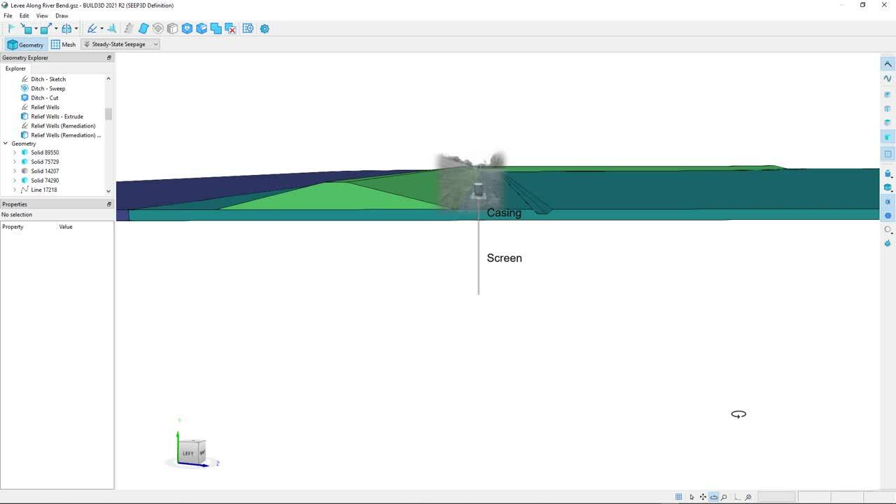
and add a schematic representation of a pressure relief well

[00:11:00.898]
onto the side of the domain.

[00:11:04.570]
Although this may look like a trash can,

[00:11:06.870]
I assure you it’s a pressure relief well.

[00:11:09.840]
The metal grill simply prevents vandalism and damage

[00:11:13.130]
to the top of the well.

[00:11:14.940]
As most of you know,

[00:11:16.500]
the well consists of a check valve

[00:11:18.320]
that prevents back flooding

[00:11:19.860]
and entrance of foreign material.

[00:11:22.480]
The casing that lies in the blanket layer is impervious,

[00:11:26.296]
whereas the screen in the aquifer allows water

[00:11:29.160]
into the well.

[00:11:30.740]
This system is relatively simple if not simplistic

[00:11:34.600]
and allows water to flow into the screen, up the well,

[00:11:38.620]
and out of the top of the well.

[00:11:41.670]
The head loss in the well

[00:11:42.930]
is generally considered negligible.

[00:11:45.350]
And the total head of the screen portion of the well

[00:11:47.950]
that lies in the aquifer

[00:11:49.690]
is set equal to the elevation at the top of the well.

[00:11:54.670]
A look at one of the wells reveals

[00:11:57.290]
that the boundary condition has been set equal

[00:11:59.620]
to a specified value of head

[00:12:01.910]
which corresponds to the elevation

[00:12:03.870]
at the top of that specific well.

[00:12:08.010]
It should be noted that we have increased

[00:12:11.130]
the mesh density along each well

[00:12:13.330]
and thus increase the mesh density

[00:12:15.210]
in the vicinity of the well

[00:12:16.930]
where hydraulic gradients are likely to be quite high.

[00:12:22.410]
If we now rotate the geometry,

[00:12:24.930]
we can see all the wells,

[00:12:27.040]
and more specifically, the screen portions of the wells

[00:12:30.470]
that extend into the aquifer.

[00:12:36.980]
So we’ve finished creating the geometry,

[00:12:39.160]
assigning materials,

[00:12:40.440]
and ascribing boundary conditions,

[00:12:42.470]
and we need to generate the mesh.

[00:12:44.820]
This is specific to our three-dimensional products

[00:12:47.370]
in which meshing is done on demand and not automatically.

[00:12:51.570]
So let’s switch over to the mesh view

[00:12:53.750]
and review the mesh that has already been created.

[00:12:59.340]
In this particular case,

[00:13:01.040]
the edge length was set equal to 30 feet,

[00:13:04.100]
which resulted in a mesh of approximately 150,000 nodes

[00:13:08.670]
and 900,000 elements.

[00:13:11.760]
If we relaunch the mesh process

[00:13:13.630]
by clicking on the OK button,

[00:13:15.810]
we see that the mesh is created in less than 20 seconds.

[00:13:39.410]
A review of the mesh quality reveals

[00:13:41.700]
that the elements are very good in the aquifer,

[00:13:44.150]
the region of interest,

[00:13:45.730]
and fair in the remainder of the domain.

[00:13:52.130]
So we’re now ready to close the editor

[00:13:54.260]
and solve the analysis.

[00:13:56.210]
Although the analysis solves in a manner of minutes,

[00:13:58.950]
the process has been edited out of the presentation

[00:14:02.370]
due to time considerations.

[00:14:07.020]
Now that the analysis has been solved,

[00:14:08.890]
we can have an in-depth look at the results.

[00:14:11.370]
But before we do so,

[00:14:12.800]
let’s close their grid and remove the edge painting.

[00:14:20.300]
The software provides the ability

[00:14:21.930]
to generate contour surfaces of a number of variables,

[00:14:24.890]
including but not limited to, total head,

[00:14:28.300]
pressure head, hydraulic radiant, flux,

[00:14:31.140]
and hydraulic conductivity.

[00:14:35.220]
Let’s start by having a look

[00:14:36.640]
at the total head contour surfaces.

[00:14:40.180]
A very nice and useful feature is the ability

[00:14:43.020]
to change the opacity of the contours in specific solids.

[00:14:51.850]
In so doing, we quickly realize

[00:14:54.040]
that large values of total head appear

[00:14:56.160]
in neuralgic portions of the aquifer

[00:14:58.650]
and more specifically, on the land side of the levee

[00:15:01.620]
near the river bend

[00:15:03.050]
and near the Eastern segment of the levee.

[00:15:09.860]
If we toggle over to the vertical gradient contour surfaces,

[00:15:14.700]
we immediately note that the higher values of total head

[00:15:17.980]
have led to large gradients below the ditch

[00:15:20.550]
and at the toe of the levee near the 90 degree bend.

[00:15:28.330]
These gradients definitely warrant further investigation.

[00:15:31.860]
The vertical gradients through the blanket

[00:15:34.090]
at the position of the ditch

[00:15:35.500]
can be determined by extracting the total head

[00:15:38.300]
at points on the bottom surface of the blanket.

[00:15:41.220]
To do so, we must first open the three-dimensional editor,

[00:15:45.583]
move over to the mesh view,

[00:15:48.000]
and define a location that contains the points.

[00:15:54.360]
This location can then be used

[00:15:56.370]
in the draw graph functionality.

[00:16:03.700]
The data provided in the graph can then be extracted

[00:16:06.970]
and pasted into a spreadsheet software.

[00:16:15.170]
The vertical gradient computed as the head loss

[00:16:18.020]
across the blanket

[00:16:19.230]
is found to exceed the critical gradient,

[00:16:21.420]
which is approximately equal to one over a large portion

[00:16:24.940]
of the ditch.

[00:16:26.090]
This is quite problematic and can be addressed

[00:16:28.430]
by adding remediation wells.

[00:16:30.520]
But before doing so,

[00:16:32.060]
let’s extract the total head data at the top of the aquifer.

[00:16:35.800]
This data will serve as a reference

[00:16:38.070]
when we compute the drawdown associated

[00:16:40.300]
with the remediation wells.

[00:16:42.970]
This is quite easy

[00:16:44.210]
and can be done by selecting the total head contours,

[00:16:47.710]
setting the opacity of all of the solids

[00:16:50.300]
except for that of the aquifer equal to zero,

[00:16:56.450]
selecting the top surface of the aquifer,

[00:16:59.110]
and clicking on the expert data by Nodes button.

[00:17:03.410]
The data can be exported in CSV or TXT formats.

[00:17:08.880]
It is important to note that the functionality

[00:17:11.070]
is only accessible when a point, line, surface

[00:17:14.820]
or solid is selected.

[00:17:18.180]
Now that we’ve exported the data,

[00:17:20.400]
we can add a number of remediation wells.

[00:17:23.150]
To do so, we need to open the three-dimensional editor,

[00:17:27.600]
select the X-Z plane,

[00:17:29.450]
sketch the points on the plane,

[00:17:52.450]
and translate the plane upwards

[00:17:54.230]
to the elevation of the bottom of the blanket.

[00:18:03.970]
Once this is completed,

[00:18:05.260]
we can extrude the wells into the aquifer.

[00:18:24.510]
We can then select each edge,

[00:18:26.660]
set the element edge,

[00:18:28.170]
and assign the boundary conditions.

[00:19:02.250]
We are then ready to mesh and solve.

[00:19:04.670]
This process has been edited out of the presentation

[00:19:07.510]
for the sake of expediency.

[00:19:09.400]
So what is the effect of the remediation wells?

[00:19:14.900]
Well, firstly, the total head contour surfaces

[00:19:18.170]
no longer extend into the aquifer near the river bend.

[00:19:28.490]
The vertical gradient below the ditch

[00:19:30.760]
is also much smaller in the vicinity of the bend,

[00:19:33.870]
but remains unmanaged near the eastern segment of the levee.

[00:19:40.200]
Moving over to the Draw Graph functionality,

[00:19:45.580]
and extracting, pasting the data into the spreadsheet,

[00:19:49.010]
shows that the vertical gradient no longer exceeds

[00:19:51.740]
the critical gradient near the river bend.

[00:19:59.180]
A clear picture of the effect of the additional wells

[00:20:02.280]
can be assessed by extracting the total head

[00:20:04.890]
at the top of the aquifer and using it

[00:20:07.950]
to draw a drawdown map.

[00:20:14.860]
As before, the data is extracted

[00:20:17.260]
by setting the opacity of all of the solids

[00:20:19.860]
except for the aquifer equal to zero,

[00:20:22.960]
selecting the top surfaces of the aquifer,

[00:20:25.960]
and clicking on the export data by Nodes button.

[00:20:46.150]
A number of different tools can be used

[00:20:47.990]
to manipulate the data and create the draw down map.

[00:20:51.660]
The tool that I really like is Python.

[00:20:54.140]
And why is that?

[00:20:55.360]
Well, first of all, it’s free and open source,

[00:20:57.890]
which is great,

[00:20:59.280]
and it’s also easy to read, learn, and write,

[00:21:02.500]
and offers a vast number of libraries.

[00:21:05.460]
The objective here is not to show you

[00:21:07.540]
how to install or program in Python,

[00:21:09.940]
but to provide the rudiments needed

[00:21:11.610]
to read-in results and create a drawdown map

[00:21:14.120]
in a manner of minutes.

[00:21:16.610]
Although Python can be downloaded

[00:21:18.230]
from the python.org website,

[00:21:20.660]
I strongly recommend installing a Python distribution,

[00:21:24.240]
such as Anaconda,

[00:21:25.518]
which will greatly simplify package management.

[00:21:30.530]
I also recommend installing

[00:21:32.210]
an integrated development environment,

[00:21:34.950]
such as PyCharm, Spyder, PyDev, IDLE or Wing,

[00:21:39.260]
which simplifies editing, running, and debugging.

[00:21:43.030]
So let’s open the script file

[00:21:44.650]
that has been saved in the folder containing the data

[00:21:47.430]
and review the eight steps needed

[00:21:49.240]
to generate the drawdown map.

[00:21:52.250]
The first step in the process

[00:21:53.840]
is to import the modules needed to accomplish

[00:21:56.500]
the desired tasks.

[00:21:58.500]
In this case, we need numpy to create tick mark

[00:22:01.600]
and level arrays,

[00:22:03.070]
CSV to read in the data,

[00:22:05.670]
and matplotlib to create the drawn on map.

[00:22:08.950]
We can then define a series of lists

[00:22:11.100]
that will contain the coordinates, model results

[00:22:14.040]
and computed values of drawdown.

[00:22:17.970]
Once this is completed,

[00:22:19.230]
we can open this CSV file of the original analysis

[00:22:22.560]
without remediation wells and read-in each line of the file

[00:22:26.570]
except for the header.

[00:22:29.360]
We can then repeat the process for the second file

[00:22:32.080]
without reading the coordinates.

[00:22:38.550]
We can then pair each item in the lists

[00:22:41.050]
that contain the values of total head using the zip function

[00:22:44.530]
and compute the draw down for each pair.

[00:22:48.490]
We are now ready to create the figure

[00:22:50.290]
that will contain the contour plot.

[00:22:52.440]
To do so, we can define the limits of the X and Y axes,

[00:22:56.540]
define an aspect ratio, generate the figure,

[00:22:59.810]
and add a title using matplotlib.

[00:23:03.750]
We can then set the limits of the X and Y axes,

[00:23:07.010]
add evenly spaced tick marks and labels

[00:23:09.180]
using the arange function provided in numpy,

[00:23:12.410]
and add titles to the axes.

[00:23:17.720]
We can then add field contours

[00:23:19.550]
on an unstructured triangular grid

[00:23:21.930]
using the tricontourf function

[00:23:24.380]
and add a color bar with ticks and title.

[00:23:28.210]
The final step in the process consists

[00:23:30.670]
in adding contour lines using the tricontour function.

[00:23:36.310]
We can then run the script by clicking on the green arrow.

[00:23:42.270]
And voila!

[00:23:43.650]
We have a drawdown map with contours, contour lines,

[00:23:47.150]
color bar, and title.

[00:23:49.040]
It should be noted that there are thousands of color maps

[00:23:51.690]
to choose from.

[00:23:53.160]
The drawdown map can be used to create

[00:23:55.110]
a smooth creative and insightful representation

[00:23:58.260]
of the effect of the remediation wells.

[00:24:00.780]
As shown in the slide,

[00:24:02.230]
the effect of the additional wells

[00:24:03.750]
is limited to the extent of the wells,

[00:24:05.780]
but extends well into the land side

[00:24:07.710]
and riverside portions of the aquifer.

[00:24:10.890]
Let’s now move on to the second example

[00:24:13.000]
that focuses on a deep well system for a 770 foot long,

[00:24:17.500]
370 foot wide and 40 foot deep excavation

[00:24:21.920]
in a 90 foot deep unconfined sandy aquifer.

[00:24:25.320]
The de-watering system consists of 12 pumping wells

[00:24:28.500]
located five feet from the crown of the excavation slopes.

[00:24:32.430]
The screen portions of the wells are 10 inches in diameter

[00:24:36.440]
and 34 feet long.

[00:24:39.160]
Each centrifugal pump has a pumping rate

[00:24:42.220]
of 1,150 gallons per minute

[00:24:45.340]
or 2.56 cubic feet per second.

[00:24:48.950]
As with most of the watering problems,

[00:24:51.150]
this problem is undeniably three-dimensional.

[00:24:53.990]
So let’s go ahead and open Seep3D,

[00:24:56.530]
review the current analysis,

[00:24:58.270]
and create a drawdown map.

[00:25:01.930]
As shown in the Project Explorer

[00:25:03.890]
on the left-hand side of the screen,

[00:25:05.870]
a three-dimensional geometry named “excavation”

[00:25:09.170]
has been used to set up the model domain.

[00:25:12.350]
The geometry is a very simple,

[00:25:14.530]
but very large 20,000 foot long,

[00:25:17.260]
11,000 foot wide and 90 foot high cuboid

[00:25:21.830]
that allows us to capture the full effect of the river.

[00:25:25.860]
Toggling off the material shading reveals the wells

[00:25:29.050]
in the cylindrical bodies or liners

[00:25:31.770]
that were used to increase mesh density

[00:25:34.110]
in the vicinity of the wells.

[00:25:37.480]
Opening the boundary condition definitions reveals

[00:25:40.830]
that the pumping flow rate was converted

[00:25:43.190]
into a prescribed flux with associated perimeter.

[00:25:47.704]
If we open the three-dimensional editor

[00:25:50.630]
and select one of the wells,

[00:25:52.670]
we see that the edge length has been set equal to five feet.

[00:25:59.120]
A look at the mesh shows an increase in mesh density

[00:26:02.700]
in the vicinity of the wells

[00:26:04.870]
which is mostly due to the presence

[00:26:06.740]
of the meshed cylindrical bodies.

[00:26:09.620]
We are now ready to close the editor and solve the analysis.

[00:26:13.470]
Although the analysis solves in a manner of minutes,

[00:26:16.150]
the process has been edited out of the presentation

[00:26:19.220]
due to time considerations.

[00:26:22.240]
Now that the analysis has been solved,

[00:26:24.230]
we can have an in-depth look at the results.

[00:26:26.830]
But before we do so,

[00:26:28.470]
let’s remove the grid and the edge painting.

[00:26:33.060]
Toggling on the total head contour surfaces

[00:26:35.660]
and changing the opacity of the solids

[00:26:38.030]
reveals a significant drop in total head

[00:26:40.670]
in the vicinity of the pumping wells.

[00:26:51.930]
The effect of the pumping wells on their phreatic surface

[00:26:54.900]
can also be assessed by defining an ISO surface.

[00:27:04.470]
The shape of their phreatic surface or ISO surface

[00:27:07.600]
is more clearly defined when adding contour lines

[00:27:10.730]
and labels.

[00:27:19.500]
A very nice and useful feature

[00:27:21.230]
is the ability to add a clipping plane

[00:27:23.360]
at the center line of the excavation.

[00:27:28.750]
A clear picture of the effect of the wells can be assessed

[00:27:31.800]
by extracting the elevation of the phreatic surface

[00:27:34.780]
and using it to draw a drawdown map.

[00:27:38.270]
To do so,

[00:27:39.103]
the clipping plane is suppressed.

[00:27:42.310]
The grid cell size is set equal to 10 feet.

[00:27:48.230]
And the data is extracted using the export results

[00:27:51.120]
by Grid Sampling button.

[00:28:10.670]
The drawdown map is created with a slightly modified script

[00:28:14.320]
in which drawdown is computed

[00:28:15.850]
as the difference between the initial elevation

[00:28:18.170]
of the phreatic surface

[00:28:19.660]
and the final elevation of the phreatic surface.

[00:28:22.800]
For the sake of clarity,

[00:28:24.400]
we’ve also added a contour line at 35 feet

[00:28:27.360]
which corresponds to the bottom of the excavation.

[00:28:31.220]
Running the script reveals that the drawdown

[00:28:38.610]
is sufficient for excavation to proceed.

[00:28:41.720]
This was a desired outcome

[00:28:43.600]
and was very easily identified using the thicker line

[00:28:47.370]
that appears in the drawdown map.

[00:28:51.230]
In this webinar,

[00:28:52.690]
a short review of the watering systems was presented,

[00:28:56.950]
two three-dimensional groundwater de-watering problems

[00:28:59.730]
were presented, reviewed, and interpreted,

[00:29:03.910]
and a simple and efficient mean

[00:29:05.710]
of creating insightful drawdown maps was presented.

[00:29:09.920]
We have now reached the end of this webinar.

[00:29:12.320]
A recording of the webinar will be available to view online.

[00:29:16.340]
Please take the time to complete the short survey

[00:29:18.760]
that appears on your screen

[00:29:20.340]
so we know what types of webinars

[00:29:22.220]
you’re interested in attending in the future.

[00:29:25.210]
Thank you very much for joining us

[00:29:26.960]
and have a great rest of your day.

[00:29:29.330]
Goodbye.