


Introduction
Landslide risk assessment and management is a common aspect of the geotechnical engineering profession. One key aspect of the risk assessment process is to evaluate the probability of failure. This example highlights the SLOPE/W probabilistic capabilities in the context of a published case history of the James Bay hydroelectric project.
Background
James Bay Case Study
The James Bay hydroelectric project in Northern Quebec, Canada, required the construction of approximately fifty kilometers of dykes on soft and sensitive clay. Divergent views were prevalent regarding the selection of appropriate factors of safety and the selection of strength properties. Due to the complexity of the geotechnical problems, an international committee was formed to address and resolve the issues (Christian et al. 1994). The issues were studied and analyzed extensively and the project has consequently become an important and often-cited case history.
The uncertainties and spatial variability in the soil properties have been documented by Ladd (1983 and 1991). Christian et al. (1994) used this data for doing a probabilistic stability analysis. El-Ramly (2001) also used this case history as part of a Ph.D. dissertation at the University of Alberta. This work has also been highlighted by El-Ramly, Morgenstern and Cruden (2002).
Spatial Variability in SLOPE/W
Spatial variability in the soil properties can be an important consideration in certain cases. This is particularly true when the potential slip surface is relatively long within one stratigraphic unit. The Monte Carlo scheme in SLOPE/W involves numerically sampling the statistical variables numerous times. The sampling can be controlled by optionally excluding or including spatial variability in the analysis.
If spatial variability is included, the sampling is controlled by changes in material types and a user-specified distance. Consider the diagram in Figure 1. There are a total of 27 slices. Slices 1, 2 and 3 are in the fill material. Slices 4 and 27 are in the crust. Slices 5, 6 and 7 are in the marine clay on the left and Slices 24, 25 and 27 are in the marine clay on the right. Slices 8 to 23 inclusive are in the lacustrine clay.
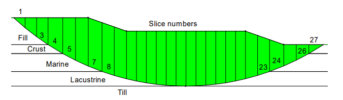
Figure 1. Slice numbers in the slide mass discretization.
If spatial variability is not selected in SLOPE/W, all of the statistical parameters are sampled once for each material. Figure 2 shows an example of the strength (cohesion) distribution for three Monte Carlo runs. The strength of slices 8 to 23 is constant for each run, but varies from run to run. Worth noting is that for 30,000 Monte Carlo runs, there would be 30,000 different strength profiles such as in Figure 2.
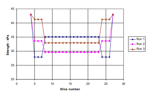
Figure 2. Example of strength variation along slip surface with no spatial considerations.
In contrast, the statistical parameters are sampled within a material multiple times when the spatial variability option is selected. SLOPE/W tracks the distance along the slip surface and when the distance exceeds the specified sampling distance, the properties are sampled. If the last sampling segment along the slip surface within one soil is shorter than the specified distance, the strength is correlated with the previous segment as described by Krahn (2004). The procedure involves local averaging as described by El-Ramly et al. (2002).
Consider the case when the sampling distance is specified as 30 m for the slip surface shown in Figure 1, which is 80 m in length. The strength of slices 8 to 23 changes each time a distance of 30 m is exceeded (Figure 3). This results in three different strengths being sampled over the 80 m.
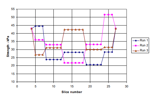
Figure 3. Variation in the clay strengths with a specified sampling distance of 30 m.
In SLOPE/W, the properties are sampled only once for a particular soil if the specified sampling distance is greater than the actual length of the slip surface within that soil. For example, the material property would be a constant for each Monte Carlo run if the sampling distance is specified as 100 m for a 90 m long slip surface. However, the strengths would be different within the same material for the left and right slip surface segments, since the properties are sampled each time the slip surface passes into a different material.
Numerical Simulation
The proposed design frequently cited in publications for James Bay is presented in Figure 4. The embankment height is 12 m with 3:1 side slopes and a 56 m wide berm at mid-height. On average, the first 4 m below the ground surface is a clay crust. Below this surface layer is a marine clay layer 8 m thick, and below this is a stratum of lacustrine clay. The lacustrine clay thickness varies depending on the depth to the till. The average depth to the till is 18.5 m, making the lacustrine clay about 6.5 m thick. The underlying till strength is high relative to the clays; consequently, the till is not relevant to the stability analysis.
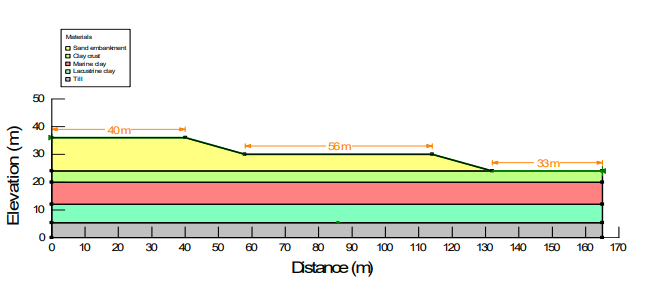
Figure 4. James Bay configuration for stability analysis.
The main factor governing stability is the strength of the soft marine and lacustrine clays. The strength was measured at 1-m depth intervals at numerous locations by field vane test. Of concern was the large scatter in the strength measurements. The mean undrained strength was found to be about 35 kPa and 31 kPa for of the marine clay and lacustrine clay, respectively.
The dispersion in the relevant data has been quantified by Ladd et al. (1983) and Christian et al. (1994). Table 1 gives the mean and standard deviations for each of these variables, which included:
- Unit weight of the embankment sand;
- Friction angle of the embankment sand;
- Thickness of the clay crust;
- Undrained strength of the marine clay;
- Vane test correction factor for the marine clay;
- Undrained strength of the lacustrine clay;
- Vane test correction factor for the lacustrine clay; and,
- Depth to the till below the ground surface.
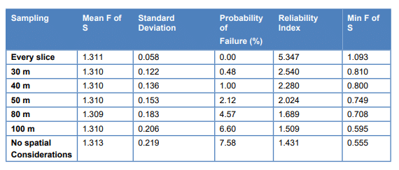
Table 1. Mean and standard deviation values.
All of the variables are assumed to have a Normal distribution. The distributions were truncated at ± 3 standard deviations for the crust thickness, the depth to the till, and the marine and lacustrine clay undrained strengths. This is necessary to avoid negative strength values and overlapping or elimination of the soil layers. The truncation is the same as adopted by El-Ramly et al. (2002). Examples of the probability distributions used in SLOPE/W are shown in Figure 5. It should be noted that the x-axis represents the offset from the mean.
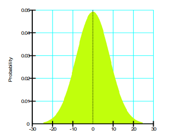
Figure 5. Probability distribution for the marine clay.
SLOPE/W cannot accommodate all of the above statistical parameters. The parameters that cannot be considered formally in the analysis are the variable crust depth, the variable depth to the till, and the variability in the vane correction factors. These uncertainties can be considered indirectly, as discussed later.
The strength of the clay crust is considered to be a constant of 43 kPa. Other constant soil properties include the unit weights of foundation clays, which are 18.8, 18.8 and 20.3 kN/m3 for the crust, marine clay, and lacustrine clay, respectively (Christian el al. 1994).
There are a total of eight analyses in the GeoStudio Project that are used to explore the effect of spatial variability on the probability of failure. All stability analyses use the Bishop method in order to compare to the publication. The first analysis establishes the deterministic FOS. Analyses 2 through 7 changes the sampling distance from ‘every slice’ up to sampling ‘every 100 m’ (e.g. Figure 6). The eighth probabilistic analysis does not consider spatial variability.
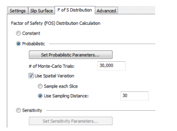
Figure 6. Spatial variability settings with a 30 m sampling distance.
Results
Deterministic Result
The previous studies by Christian el al. (1994) and El-Ramly et al. (2002) consider that the critical mode of failure is a circular slip surface that extends down to the till surface as illustrated in Figure 7. It should be noted, however, that their analyses considered the variability in the depth to the till, so the probability results included various slip surface positions. The SLOPE/W deterministic Bishop Factor of Safety for the slip surface shown in Figure 7 is 1.460. This is the same value computed by others in previous studies. Christian el al. (1994) computed a value of 1.453 and El-Ramly et al. (2002) computed a value of 1.46
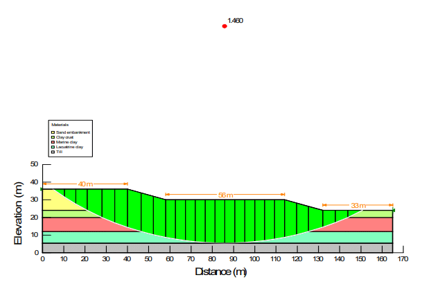
Figure 7. Shape and position of critical slip surface.
Probabilistic Results
Table 2 presents the probability distribution characteristics for each case of spatial variability. The highest probability of failure occurs for Case 8, which does not consider spatial variability (1.34%). This occurs because sampling within each material once per run makes it possible to have all the parameters at the lowest value at the same time. This also results in the lowest possible minimum factor of safety.
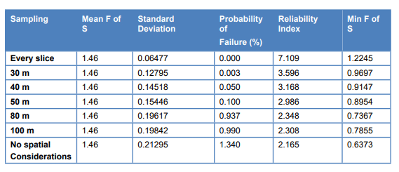
Table 2. Probability of failure as a function of sampling distance.
The lowest probability of failure occurs when sampling the statistical parameters for every slice. In fact, the lowest of the 30,000 computed factors of safety was 1.2245 and the probability of failure is 0.0. Sampling the statistical properties for every slice does not likely give a realistic picture of uncertainty. It is somewhat analogous to creating a probability density histogram. If the interval becomes too small, it is difficult to detect a distribution of any quantifiable shape. The same problem exits if the interval is too high. The feature is nonetheless available in SLOPE/W as a convenient way of bracketing the lower end of a range in probability of failure. Allowing for no spatial variability tends to bracket the upper end of the range.
There is a slight difference in the probability of failure between sampling distances of 30 m and 50 m and a marginal increase for distances of 80 and 100 m. The fact that all probabilities of failure are less than 1.0 % when some form of spatial variability is considered may be a more important observation than the range in values. More importantly, perhaps, is the issue in the difference between none versus some spatial variability.
Vane strength corrections
Christian et al. (1994) and El-Ramly et al. (2002) included a vane strength correction as one of the statistical parameters for the marine clay and the lacustrine clay. SLOPE/W does not allow for a modification distribution function to be applied to a soil property distribution function. The vane corrections could, however, be included in an approximate way by correcting the field measurements before computing the mean and standard deviation. The correction would then be included indirectly in the soil property distribution function. Presumably, the mean and standard deviation would be different for the corrected and uncorrected data sets.
Effect of geometric variability
Christian et al. (1994) and El-Ramly et al. (2002) also included variations in the clay crust thickness and in the depth to the till. Varying the depth to the till alters the thickness of the lacustrine clay and the position of the slip surface. This has a significant effect, because such a large portion of the slip surface is within the lacustrine clay. A deeper slip surface means a larger portion of the slip surface length is in lacustrine clay, which is the weakest material.
The variable soil thicknesses cannot be considered statistically in SLOPE/W, but the effect can be considered by looking at various configurations and potential slip surfaces. The average thickness of the clay crust is 4 m, with a standard deviation of about 0.5 m. If we consider the truncation of three standard deviations as a limit, the clay crust could be as thin as 2.5 m. The standard deviation on the depth to the till is 1.0 m. Again, with a truncation of three standard deviations as a limit, the depth to the till could be as much as 21.50 m. This configuration is shown in Figure 10. Figure 11 shows the position of the critical slip surface. The deterministic factor of safety is 1.310, which is about 15 % lower than for the average conditions presented above.
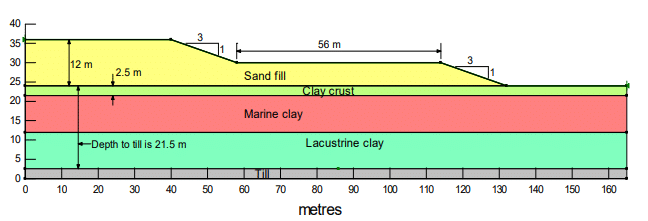
Figure 10. Configuration with thin crust and thick lacustrine clay.
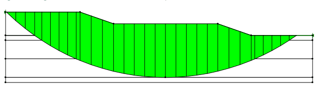
Figure 11. Position of slip surface with thin crust and thick lacustrine clay.
Table 3 shows the probabilistic parameters for the altered geometry. The probabilities of failure are now significantly higher. At a 30-m sampling distance, for example, the increase is from 0.003% up to 0.48%. The probability of failure increases from 1.34% up to 7.58% for the case without spatial variability.
Table 3. Probability parameters with thin crust and thick lacustrine clay.
The increases in the probabilities of failure are a direct reflection of the lower deterministic factor of safety, or a direct reflection of a more critical mode of failure. As discussed below, this follows a usual trend that the higher probabilities of failure occur for the deterministically most critical slip mode.
Comparison with published analyses
It is difficult to make a direct comparison with the results presented by others, because the details are different in each study. The closest is the study by El-Ramly et al. (2002). SLOPE/W follows the sampling distance concepts presented in this study. El-Ramly et al. (2002) used three sampling segments in the lacustrine clay, two in the marine clay and four in the embankment. The depth to the till was included as a variable and, given that the geometric variation significantly increases the probability of failure, the closest condition to the El-Ramly analysis is the one with the thick lacustrine clay and a 30-m sampling distance. For this condition, the comparison between these two analyses is as listed in Table 4.
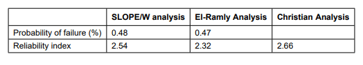
Table 4. Comparison of different analyses.
Christian el al. (1994) did a first-order second moment (FOSM) type of analysis. Their reliability index for a comparable situation is 2.66, as shown in Table 4. The probability of failure was not listed in the study. In spite of the differences in all three studies, the findings are remarkably close. This demonstrates that the SLOPE/W formulation gives results comparable with other different and independent analyses.
Discussion
If sufficient data is available, a variogram can be determined, as discussed by Soulié et al. (1990). The form of a variogram is illustrated in Figure 12. The differences in strength, for example, increase with distance between sampling points up to a certain distance, after which the difference remains constant. The point at which the variogram becomes horizontal is called the range, and it is the distance beyond which there is no correlation between strength measurements. The range from a variogram would be an appropriate sampling distance for a SLOPE/W probabilistic analysis.
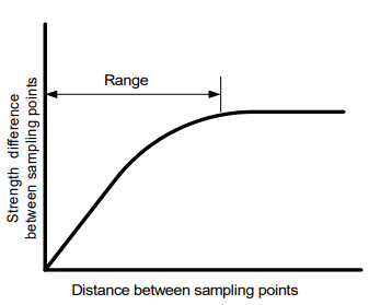
Figure 12. A typical variogram.
Unfortunately, sufficient data is seldom available to formally evaluate the spatial variability, and so it comes down to making a judgment. Making an intuitive judgment, however, may be better in some cases than ignoring the possibility of spatial variability completely. El-Ramly et al. (2002) go so far as to say that ignoring spatial variability, “… can be erroneous and misleading.” This may be overstating the case for some analyses, but it does highlight the importance of giving spatial variability its due consideration in an analysis. SLOPE/W can facilitate this type of analysis because various sampling distances can be examined easily and quickly.
An important point to note in the Christian et al. (1994) and the El-Ramly et al. (2002) studies is that the slip surface position is tied to the till elevation. This is likely reasonable because the undrained strengths of the clays are assumed to be constant with depth, which causes the critical slip surface tends to go as deep as possible. In many situations the soil strengths tend to increase with depth and the position of the critical surface may then be somewhere within the soil stratum. Including geometric variability for such a situation becomes much more complicated. The best way to handle this in SLOPE/W is to do a probabilistic analysis on multiple slips surfaces. An option is available to do a probabilistic analysis on a user-selected number of slip surfaces closest to the most deterministically critical slip surface.
Summary and Conclusions
The James Bay probabilistic studies have shown the important effect of including spatial variability in an analysis. It is particularly important for this case because of the relatively long slip surface, especially in the lacustrine clay. It seems unreasonable to assume that this clay would have the lowest strength predicted from the probability distribution over the entire distance of the slip surface, especially considering the large scatter in the field measurements.
The big attraction of a tool such as SLOPE/W is the ease with which probabilistic analyses can be performed. Once a problem has been set up for a deterministic analysis, there is very little extra modeling effort involved in doing a probabilistic analysis. No extra tools are required. A variety of probabilistic distribution functions are available with truncation as necessary. Even a general data point distribution function is available for any unusual distribution of properties. The most difficult part of the analysis is obtaining sufficient data to define the dispersion appropriately.
References
Christian, J.T., Ladd, C.C. and Baecher, G.B. (1994). Reliability and probability in stability analysis. Journal of Geotechnical Engineering, ASCE, Vol. 120, pp. 1071-1111.
El-Ramly, H. (2001). Probabilistic analyses of landside hazards and risks: bridging theory and practice. Ph.D. Thesis, University of Alberta, Edmonton, Alberta, Canada
El-Ramly, H., Morgenstern, N.R. and Cruden, D.M. (2002). Probabilistic slope stability analysis for practice. Canadian Geotechnical Journal, Vol. 39, No. 3, pp. 665-683.
Krahn, J. (2004). Stability Modeling with SLOPE/W, An Engineering Methodology, First Edition, Prepared and printed in-house by GEO-SLOPE International Ltd, Calgary, Alberta, Canada
Ladd, C.C. (1983). Geotechnical exploration in clay deposits with emphasis on recent advances in laboratory and in situ testing and analysis of data scatter. Journal of Civil and Hydraulic Engineering, Taiwan, 10(3), pp. 3-35.
Ladd, C.C. (1991). Stability evaluation during staged construction. Journal of Geotechnical Engineering, ASCE, 117 (4) pp. 540-615.
Soulié, M., Montes, P. and Silvestri, V. (1990). Modelling spatial variability of soil parameters. Canadian Geotechnical Journal, Vol. 27, No. 5, pp. 617-630