Industry Best Practices for UXO detection and analysis

This webinar covers:
– An overview of common challenges faced when trying to locate UXO
– How to overcome these challenges, reduce time and costs, and enhance detection accuracy

Overview

Video Transcript

[00:00:00.431]
(soft intro music)

[00:00:11.470]
<v Lorraine>Hello, everyone.</v>

[00:00:12.303]
I’d like to welcome you to today’s webinar

[00:00:14.120]
on industry best practices

[00:00:15.710]
for unexploded ordnance detection and analysis.

[00:00:18.710]
My name is Lorraine Godwin.

[00:00:19.960]
I’m the Global Business Director

[00:00:21.360]
for Seequent’s near surface and marine division.

[00:00:24.600]
Unexploded ordnance detection can be expensive, risky,

[00:00:28.450]
and time consuming to find and locate,

[00:00:30.620]
and excavation costs can quickly add up,

[00:00:33.200]
but there are industry best practices,

[00:00:35.080]
which we’re going to be talking about today.

[00:00:40.970]
All right, before I introduce our speaker,

[00:00:43.960]
I’ll take us through a little bit

[00:00:45.480]
of the GoTo webinar housekeeping.

[00:00:51.950]
You’ll notice that GoTo has a menu option

[00:00:55.200]
on the right hand side of the screen.

[00:00:56.690]
You can expand this by pressing the orange arrow,

[00:00:59.960]
and that will give you more options.

[00:01:01.750]
If you are having any audio troubles,

[00:01:03.580]
please log out and log back in,

[00:01:05.420]
or you can also select the phone call option

[00:01:07.520]
to dial in by phone.

[00:01:10.480]
To minimize the background noise,

[00:01:12.200]
we have muted everyone by default,

[00:01:14.200]
but if you have questions,

[00:01:15.190]
we do encourage you to type these into the question window

[00:01:18.180]
in the GoTo webinar control panel.

[00:01:21.690]
And we are recording today’s session.

[00:01:23.540]
The recording will be sent out following today’s webinar.

[00:01:28.140]
Seequent create powerful geoscience analysis

[00:01:30.587]
and 3D modeling software

[00:01:32.610]
that allows for integration of different geo datasets

[00:01:36.960]
to understand the subsurface of the earth.

[00:01:39.290]
The company was originally founded in the early 2000s,

[00:01:42.770]
born out of medical 3D imaging technology,

[00:01:45.360]
which in 2004 was applied to understanding

[00:01:48.540]
geological science and the subsurface of the earth.

[00:01:52.550]
These geo datasets are used to find mineral resources,

[00:01:57.410]
for looking at infrastructure and construction projects,

[00:02:00.610]
understanding the geo-technical properties,

[00:02:04.780]
oil and gas deposits, geothermal, natural hazards,

[00:02:08.040]
and looking for water resources.

[00:02:10.340]
Today, we’re a team of over 350 people

[00:02:13.220]
that includes geo scientists, engineers, researchers.

[00:02:17.180]
Our head office is in New Zealand

[00:02:18.650]
and we have 18 locations around the world.

[00:02:22.540]
The vision of the company

[00:02:23.760]
is to enable better decisions about earth,

[00:02:26.020]
environment and energy challenges using geo data

[00:02:29.080]
to understand the subsurface of the earth.

[00:02:32.680]
Today, we are focusing on

[00:02:34.180]
Seequent’s geo-physical solution platform

[00:02:37.520]
called Oasis montaj.

[00:02:39.220]
Oasis montaj is a powerful geoscience platform

[00:02:42.130]
for analyzing and interpreting geophysical data

[00:02:45.610]
and integrating it with other types of bore hole,

[00:02:48.300]
drill hole and geochemical data.

[00:02:51.180]
It’s been applied for unexploded ordnance detection

[00:02:53.830]
for over 30 years.

[00:02:57.130]
I am going to be your host for today,

[00:02:59.230]
and our speaker is Laura Quigley.

[00:03:02.560]
Laura Quigley is the technical analyst

[00:03:04.560]
with our near surface and marine division.

[00:03:07.420]
She received her Bachelor of Science degree in Geophysics

[00:03:10.900]
from Memorial University in Newfoundland

[00:03:13.540]
and her Master’s of Science degree in Geophysics

[00:03:16.020]
from the University of Toronto.

[00:03:17.930]
Her professional career started with

[00:03:19.580]
Fugro Airborne Surveys,

[00:03:21.660]
where she would process

[00:03:22.680]
and interpret airborne geophysical data.

[00:03:25.270]
She then worked for a marine seismic company

[00:03:27.370]
where she participated in a large number of research cruises

[00:03:30.390]
to Greenland.

[00:03:31.620]
After completing her master’s degree in 2013,

[00:03:35.220]
Laura moved to Australia

[00:03:36.870]
and worked in a research environment

[00:03:38.380]
with various universities in Brisbane.

[00:03:40.750]
She worked for the University of Queensland

[00:03:42.470]
on seismic projects

[00:03:43.610]
for unconventional coal seam gas development,

[00:03:46.430]
and then moved to Queensland University of Technology

[00:03:49.300]
where she spent several years researching

[00:03:51.130]
geo dynamical processes through analog modeling.

[00:03:55.020]
Laura returned to Canada in January, 2020

[00:03:57.450]
to join Seequent as our Technical Analyst

[00:04:00.070]
with our new surface and marine team.

[00:04:02.760]
Please welcome Laura Quigley.

[00:04:06.630]
<v Laura>Great. Thanks Lorraine.</v>

[00:04:08.450]
Hi everybody,

[00:04:09.283]
and welcome to this webinar about industry best practices

[00:04:12.040]
for UXO detection and analysis.

[00:04:15.010]
Why digital geophysical methods

[00:04:16.520]
are best for identifying UXO.

[00:04:21.130]
So an agenda of the webinar today is as follows.

[00:04:24.510]
I’m going to talk about what are UXO.

[00:04:28.020]
Why are they a problem.

[00:04:30.480]
Methods of detecting UXO,

[00:04:33.140]
and pros and cons of each method.

[00:04:36.120]
And then finally, some Oasis montaj solutions for UXO.

[00:04:41.170]
So what are UXO?

[00:04:43.240]
UXO stands for unexploded ordnance.

[00:04:46.070]
Other acronyms referring to the same thing

[00:04:48.270]
include UXB for unexploded bombs,

[00:04:50.910]
ERW for explosive remanence of war,

[00:04:54.370]
MEC for munitions or equipment of concern.

[00:04:58.610]
So all these acronyms refer to explosive weapons

[00:05:02.060]
that did not explode and still pose a threat of detonation.

[00:05:07.730]
So UXO is a global problem.

[00:05:09.810]
More than 80 countries are affected by UXO.

[00:05:13.120]
So this map highlights the number of UXO casualties

[00:05:15.820]
around the world with red being the most extreme.

[00:05:19.730]
Most of the UXOs are from past wars.

[00:05:21.860]
So World War I and World War II over 70 years ago.

[00:05:26.170]
Also more recent conflicts in certain parts of the world,

[00:05:28.940]
such as Vietnam, Laos, and Cambodia,

[00:05:31.800]
which were heavily bombed during the Vietnam War

[00:05:34.120]
in the 60s and 70s are highly contaminated by UXOs today.

[00:05:39.690]
In the UK alone,

[00:05:40.700]
there were still tens of thousands of tons of explosives,

[00:05:43.420]
which did not detonate from World War II.

[00:05:47.120]
And unlike parts of Europe and Asia,

[00:05:49.270]
UXO problem in the US

[00:05:50.610]
mainly comes from previous military testing sites

[00:05:53.640]
as opposed to world wars or other wars.

[00:05:57.550]
And also, UXO can be located onshore and offshore.

[00:06:04.780]
So why are UXO a problem?

[00:06:09.170]
People’s safety.

[00:06:10.580]
So today, UXO from recent conflicts, legacy wars

[00:06:14.490]
and old military training sites

[00:06:16.250]
still kill and injure thousands of people.

[00:06:19.140]
Often rural farmers have no choice, but to farm land,

[00:06:21.920]
which is contaminated by UXOs.

[00:06:24.720]
15 to 20,000 people a year are injured or killed,

[00:06:27.920]
and approximately 80% of those are civilians.

[00:06:33.880]
Another reason UXO are a problem

[00:06:35.850]
is because of the environmental hazard.

[00:06:37.740]
So environmental contamination.

[00:06:40.400]
For example, TNT was an important military explosive.

[00:06:43.660]
Red water associated with TNT pollution

[00:06:45.780]
is toxic to the environment

[00:06:47.160]
and is considered hazardous waste.

[00:06:51.850]
Also, many UXO still remain on the sea floor.

[00:06:55.490]
So this is a problem for fishing, oil and gas,

[00:06:58.470]
telecommunications.

[00:07:00.730]
So the risk of detonation,

[00:07:02.470]
as well as chemicals leaching into the ocean.

[00:07:09.380]
And finally, infrastructure and community growth

[00:07:12.580]
is affected by UXOs.

[00:07:15.640]
So cities cannot expand and grow

[00:07:18.770]
without UXO remediation and removal.

[00:07:22.160]
Previous military sites, for example, in the US

[00:07:25.000]
which were located in the middle of nowhere

[00:07:26.520]
during war times are now encroaching upon

[00:07:29.240]
areas that are being developed for residential

[00:07:31.730]
or business uses.

[00:07:33.780]
And this is a danger for both onshore

[00:07:36.140]
and offshore construction and excavation work.

[00:07:43.000]
Okay, next I’m going to show you some examples

[00:07:45.400]
of how UXO are affecting the communities today.

[00:07:49.450]
This is an onshore example.

[00:07:51.260]
So this is a recent airport closure in Germany.

[00:07:54.770]
Germany was heavily bombed during World War II.

[00:07:57.740]
So thousands of UXO from World War II

[00:07:59.940]
are uncovered each year in Germany.

[00:08:02.720]
In this particular instance,

[00:08:03.940]
a 450 kilogram bomb

[00:08:06.030]
was located on the outskirts of the city.

[00:08:08.910]
And this picture shows travelers

[00:08:10.460]
waiting outside the Hamburg Airports in 2017

[00:08:14.120]
while bomb disposal experts defuse this bomb.

[00:08:17.730]
This also resulted in evacuation of 300 homes in the area.

[00:08:26.640]
And now I’m going to show you an offshore example.

[00:08:28.840]
So this picture here shows the mast of a US cargo ship.

[00:08:32.770]
It sank in 1944 off the coast of UK.

[00:08:37.520]
So this is the SS Richard Montgomery.

[00:08:40.570]
It was carrying tens of tons of munitions

[00:08:43.720]
and they sank with the ship.

[00:08:46.250]
And all are still onboard today,

[00:08:48.170]
which is actually only 15 meters below the sea surface.

[00:08:51.800]
So it’s constantly monitors.

[00:08:54.900]
However, the removal of the munitions is just too complex

[00:08:58.970]
and dangerous at this point.

[00:09:05.040]
So who’s involved in the cleanup?

[00:09:07.700]
So much effort is

[00:09:08.670]
and continues to be put into UXO remediation.

[00:09:11.790]
It is not easy.

[00:09:13.670]
It’s often difficult to locate UXO and manage them,

[00:09:18.450]
and very costly to remove.

[00:09:21.220]
So due to these risks,

[00:09:22.840]
the removal is a joint effort between government agencies,

[00:09:26.560]
private companies, contractors,

[00:09:28.780]
as well as humanitarian groups.

[00:09:31.230]
So humanitarian groups include MAG and the HALO Trust,

[00:09:35.600]
and these groups work in developing countries

[00:09:39.230]
to help give the land back to the people.

[00:09:41.620]
So they clear land for agricultural development

[00:09:43.760]
and community purposes.

[00:09:46.070]
In the US, the Department of Defense

[00:09:48.490]
and the US Army Corps of Engineers

[00:09:50.170]
are responsible for clearing formerly used defense sites,

[00:09:54.600]
and various other private organizations and contractors

[00:09:58.380]
work around the world on UXO projects.

[00:10:05.140]
Okay, so now I’m going to talk about

[00:10:07.040]
methods for UXO detection,

[00:10:09.430]
both analog methods and digital geophysical methods.

[00:10:15.690]
So analog also known as mag and flag

[00:10:19.020]
involves hand-held metal detectors.

[00:10:21.940]
These metal detectors have been used for centuries

[00:10:24.100]
to find treasures.

[00:10:26.330]
So operators walk along the ground,

[00:10:28.060]
moving the instrument from side to side.

[00:10:30.860]
And when they either hear or see a signal,

[00:10:33.500]
they place a small pin flag in the ground,

[00:10:36.490]
and this signal is from passing over a metallic object.

[00:10:41.340]
So this results in a large number of flags,

[00:10:45.200]
all which have to be dug as it is unknown

[00:10:47.890]
what is associated with each flag.

[00:10:52.930]
Okay, so digital geophysical methods.

[00:10:55.220]
I’m going to show you some examples.

[00:10:57.380]
So for digital geophysics,

[00:10:59.440]
the two primary techniques are electromagnetic induction

[00:11:02.930]
and magnetics.

[00:11:04.950]
Data is digitally stored on a computer system.

[00:11:08.350]
So these two onshore systems shown here.

[00:11:12.300]
The one on the left is an electromagnetic conduction system.

[00:11:16.220]
It uses transmitter and receiver coils.

[00:11:19.230]
So a transmitter coil sends a signal into the ground,

[00:11:23.080]
and when it encounters a metallic object,

[00:11:25.120]
a secondary signal is generated

[00:11:27.310]
and this secondary signal is picked up by receiver coils.

[00:11:31.570]
So this method is an active method,

[00:11:35.200]
meaning you can send a signal into the ground

[00:11:38.340]
and it detects any metallic objects,

[00:11:40.600]
so ferrous or non-ferrous.

[00:11:45.788]
On the right, we have a magnetic sensor.

[00:11:48.210]
So this is a passive method.

[00:11:49.830]
It’s a method that detects any changes

[00:11:52.360]
in the earth’s magnetic fields.

[00:11:54.730]
So this works well for ferrous objects.

[00:11:57.750]
So any object that contains a high concentration of iron.

[00:12:02.320]
A lot of UXO have steel casing.

[00:12:04.700]
So this method works particularly well.

[00:12:08.250]
Okay, so now I’m going to show you some systems

[00:12:10.140]
for digital geophysics offshore.

[00:12:12.470]
So the same principles apply.

[00:12:14.010]
We have electromagnetic induction on this slide.

[00:12:16.650]
This is an EM61 sensor

[00:12:18.280]
that is now designed for offshore surveying.

[00:12:20.880]
So this is a fairly recent technology.

[00:12:28.230]
And magnetic sensors.

[00:12:29.570]
So these have been used offshore for a number of years

[00:12:32.400]
to do offshore surveying.

[00:12:34.800]
So this is a single sensor on the left,

[00:12:37.600]
a marine magnetometer,

[00:12:39.600]
and two sensors shown on the right.

[00:12:42.540]
So this is gradiometry mode for surveying.

[00:12:45.970]
This is easy to tow behind ships,

[00:12:47.850]
and you can tow just meters above the sea floor.

[00:12:53.890]
Another way of collecting UXO survey data

[00:12:57.350]
is using drones or UAVs.

[00:13:00.710]
So this picture here on the left shows the mag arrow,

[00:13:04.130]
so a magnetic sensor being operated by a drone,

[00:13:08.040]
and the picture on the right shows another system

[00:13:10.100]
known as the drone mag.

[00:13:12.210]
So this is a good option

[00:13:13.730]
for when the terrain is often difficult to walk.

[00:13:16.850]
And it can produce quite a dense dataset.

[00:13:19.880]
So with airborne surveys, line spacing is often 100 meters,

[00:13:25.860]
where with drones, you can get line spacing

[00:13:28.110]
down to just a few meters.

[00:13:32.240]
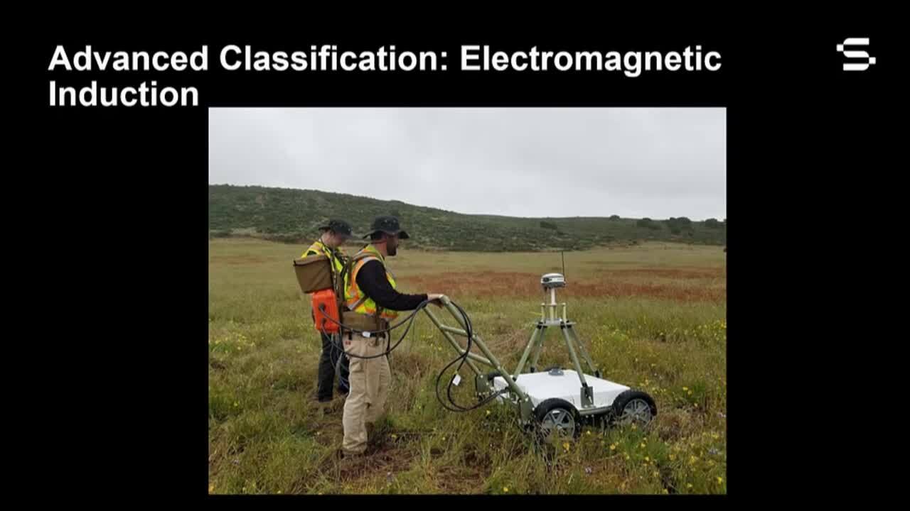
Okay, so advanced classification.

[00:13:34.870]
This is the latest digital geophysical method

[00:13:37.550]
for UXO surveying.

[00:13:39.670]
It involves electromagnetic induction, as I spoke of before,

[00:13:43.750]
the difference being it uses multiple receiver

[00:13:46.440]
and multiple transmitter coils at different orientations.

[00:13:50.510]
So a large number of information is collected

[00:13:54.870]
at each data point,

[00:13:56.560]
and this information can provide

[00:13:59.520]
the necessary properties of the target

[00:14:01.960]
that can distinguish it as a UXO or non-UXO.

[00:14:05.780]
So it has the ability to actually classify your targets.

[00:14:08.970]
And this is done based on prior knowledge of UXO signals

[00:14:15.900]
that have been recorded.

[00:14:20.950]
Okay, so now I’m going to talk about

[00:14:23.070]
the advantages and disadvantages of each method.

[00:14:26.920]
So I’ve listed on the left, mag and flag disadvantages

[00:14:30.310]
and on the right, geophysical method advantages.

[00:14:34.280]
So on the left.

[00:14:36.290]
So for mag and flag, data is not recorded,

[00:14:40.010]
and with digital geophysical methods,

[00:14:42.610]
you have all your data recorded as well as geo-referenced.

[00:14:46.790]
So you have GPS data along with all your geophysical data.

[00:14:53.220]
And mag and flag is very influenced by the operator.

[00:14:56.460]
So system sensitivity can be turned up or down.

[00:15:00.260]
Signals can be missed either audio or visual signals

[00:15:04.090]
and operator keys in the pocket or cell phones

[00:15:07.820]
can interfere with the signal.

[00:15:10.670]
And with digital geophysical methods,

[00:15:12.750]
you can have an audit trail of your data.

[00:15:14.490]
So because all the data is recorded,

[00:15:16.630]
you can go back and analyze it later

[00:15:18.860]
to see if your survey coverage was 100%,

[00:15:22.490]
make sure all the instruments were working, all the sensors.

[00:15:28.340]
So magnetic soils tend to cover up signals, UXO signals,

[00:15:33.890]
where they exist.

[00:15:35.880]
So digital geophysics can allow you to process

[00:15:38.810]
the effect of the magnetic soils from your data,

[00:15:42.730]
as well as any background geology effects can be removed.

[00:15:46.890]
So this leaves just your UXO signal clear in the data.

[00:15:51.780]
Mag and flag has a high false alarm rate.

[00:15:55.100]
So that means the number of targets flagged

[00:15:58.990]
versus the number of UXOs discovered is very high.

[00:16:03.130]
And with digital geophysics,

[00:16:04.300]
we’re able to characterize and often classify targets.

[00:16:08.090]
So this reduces the number of false alarm rates,

[00:16:10.790]
so reducing the digs.

[00:16:14.050]
And mag and flag,

[00:16:15.520]
you cannot reference flag locations to any other data.

[00:16:20.810]
With digital geophysics, each data point is geo-referenced.

[00:16:23.690]
So you can bring in other maps,

[00:16:25.540]
such as other geophysical maps or geological maps

[00:16:28.740]
to help with your interpretation.

[00:16:31.940]
Mag and flag is relatively inefficient

[00:16:33.920]
as it can scan smaller areas of land at a time,

[00:16:37.300]
and digital geophysics allows for dense datasets.

[00:16:41.480]
And then finally, for mag and flag,

[00:16:43.470]
every target needs to be dug

[00:16:45.780]
and digital geophysics allows one to compile a dig list

[00:16:49.210]
based on data analysis.

[00:16:54.890]
Okay, so now I’m going to talk about the way forward.

[00:17:03.450]
So costs associated with UXO detection and removal.

[00:17:07.800]
So this graph highlights some of the costs associated

[00:17:10.580]
with detection and removal.

[00:17:12.810]
Site assessment, survey mapping,

[00:17:15.310]
vegetation removal, scrap metal removal,

[00:17:18.360]
and UXO removal and disposal.

[00:17:20.550]
So as we can see,

[00:17:22.000]
a vast majority of the costs

[00:17:24.080]
are associated with digging up scrap metals,

[00:17:26.680]
so non-UXO targets.

[00:17:29.330]
So there’s often thousands of targets on a site,

[00:17:33.010]
which are identified for digging,

[00:17:36.340]
and each dig can cost between about 35 and 100 euros.

[00:17:40.360]
So costs add up really quickly.

[00:17:43.360]
And it’s been shown that advanced geophysical techniques

[00:17:46.700]
have stopped excavation of non-UXO targets by up to 90%.

[00:17:51.660]
And this money can be used on other projects,

[00:17:53.730]
other UXO projects.

[00:17:57.860]
So false positive ratio: Mag and flag.

[00:18:01.290]
It’s 100:1 on average.

[00:18:03.750]
So that is 100 digs that were non-UXO

[00:18:07.680]
to every one UXO discovered.

[00:18:12.770]
And with digital geophysical methods,

[00:18:15.060]
this ratio reduces to 10:1.

[00:18:21.300]
Okay, so now I’m going to go into our Oasis montaj software

[00:18:25.070]
and just show you some tools you can use for UXO processing

[00:18:28.460]
of digital geophysical data.

[00:18:33.270]
So I’ve created a project and it’s called single mag,

[00:18:36.840]
and I’m going to show you a Marine Magnetic survey

[00:18:39.410]
off the coast of Hawaii, just some sample data.

[00:18:43.520]
And I’m going to show you a lot of the processing

[00:18:45.610]
that we can do in this particular workflow

[00:18:47.770]
of UXO marine mag.

[00:18:49.800]
So I can import my data

[00:18:53.270]
and it gets imported into a database.

[00:18:56.390]
I’ll call the database, single mag_2.

[00:19:01.370]
And then you can locate your survey file,

[00:19:03.200]
which is a CSV for this particular survey.

[00:19:06.290]
And then I create a template for the imports.

[00:19:12.350]
And on the last step of the import,

[00:19:14.030]
I can tell which channels are line channel.

[00:19:17.190]
So this way the survey data is split on the line channel

[00:19:19.880]
and in the rest of the columns are channels or data type.

[00:19:26.490]
Okay, so now I have my data in a database,

[00:19:28.930]
and it’s very similar to an Excel spreadsheet.

[00:19:31.870]
However, I’m going to geo-reference my data now

[00:19:33.840]
so it knows which coordinate system it’s in.

[00:19:37.400]
And this is projected X, Y.

[00:19:39.990]
And its UTM zone for North for Hawaii.

[00:19:43.670]
And then click okay,

[00:19:45.170]
and now your data is geo-referenced

[00:19:46.890]
and you can see in the bottom

[00:19:48.010]
which coordinate system your data is in.

[00:19:52.090]
So we can see all the survey lines

[00:19:53.810]
if we right click on the top left cell.

[00:19:57.110]
There’s 57 lines in the survey.

[00:20:00.630]
We can scroll through them.

[00:20:02.820]
And I’m just going to show you a database view

[00:20:05.380]
where we use our profile windows,

[00:20:07.010]
which are available here.

[00:20:10.380]
And I have a view that’s been set up.

[00:20:15.430]
So this is a good way to check all your data.

[00:20:17.870]
I have X channel displayed on top,

[00:20:20.710]
then the Y channel, then the magnetics channel,

[00:20:23.410]
and the altitude on bottom.

[00:20:26.520]
And I can scroll through my lines and check for any errors,

[00:20:29.450]
any dropouts, any spikes.

[00:20:33.690]
So now I’m going to show you how to correct for the X and Y,

[00:20:36.270]
which is the GPS positions.

[00:20:39.320]
Any spikes, any dropouts, any errors in the GPS.

[00:20:43.060]
So we go to UXO marine mag and we do a path correction.

[00:20:47.820]
I just tell it which database to look in,

[00:20:49.890]
and it’ll create a backup of my X and Ys.

[00:20:53.680]
And then I click, okay.

[00:20:58.230]
This also produces a map

[00:20:59.770]
and the map shows you your survey coverage,

[00:21:02.370]
which is a really great tool.

[00:21:07.460]
Okay, so here’s my survey lines with the corrected GPS data,

[00:21:12.020]
X and Y data.

[00:21:14.090]
And we can overlay some aerial imagery

[00:21:16.500]
using our seek data, add bing imagery tool.

[00:21:22.900]
So this aerial data is just a really good way

[00:21:24.750]
to interpret your data

[00:21:27.360]
to see if the coverage was where you thought it was.

[00:21:29.980]
However, it doesn’t export with any final products.

[00:21:33.950]
Okay, so we see our survey was in the marine environment.

[00:21:37.120]
There’s some man-made structures.

[00:21:38.410]
So there’s a dock and it was off the coast of Hawaii.

[00:21:44.130]
Okay, so now I’m going to close this.

[00:21:47.970]
And I can always come back to it

[00:21:49.230]
if I wanted to use it for interpretation purposes.

[00:21:53.170]
Next, I’m going to show you some magnetics data,

[00:21:55.360]
which I’ve processed.

[00:21:57.370]
And I’m going to use a different database that I’ve worked on.

[00:22:02.940]
So that’s the same data just with some processing done.

[00:22:06.330]
So in the UXO marine mag menu,

[00:22:08.460]
we can process data for altimeter corrections,

[00:22:12.750]
and we can also model the background’s magnetic fields,

[00:22:16.240]
which we can then remove from our data.

[00:22:18.960]
So the top profile window here shows the magnetics

[00:22:22.210]
before and after an altitude correction.

[00:22:25.090]
So before the altitude correction is the blue curve

[00:22:27.140]
and after is the red curve.

[00:22:29.000]
In the middle profile I’ve shown the altimeter.

[00:22:31.700]
And this is just a good way to see

[00:22:33.540]
if our data correction did what we thought it should do.

[00:22:37.340]
So it’s actually, the altimeter is slightly higher here.

[00:22:41.150]
So it’s actually brought my anomaly up a bit.

[00:22:46.300]
And the bottom profile we’re now showing here

[00:22:49.310]
is just the magnetics data with a modeled background field

[00:22:53.260]
shown in green.

[00:22:54.910]
So we can use this modeled background fields

[00:22:58.200]
to subtract from our magnetics data,

[00:23:00.910]
leaving just the anomalies of interest.

[00:23:03.970]
And all this was done in the data corrections tool.

[00:23:11.380]
Okay, so that’s my data in profile view.

[00:23:13.270]
Next, I’m going to talk about grids.

[00:23:15.820]
So we can grid our data.

[00:23:17.850]
So this interpolates the magnetics

[00:23:19.810]
or anything we choose to grid between survey lines.

[00:23:23.580]
And I’m going to show you my grids on a map.

[00:23:26.110]
So you can drag any of these grids onto a map window.

[00:23:29.510]
It’s just a nice way to display your data.

[00:23:31.430]
You get a North arrow, scale bar and you can add a title.

[00:23:35.920]
So I’m going to show you.

[00:23:36.753]
This is the magnetics data I processed.

[00:23:39.090]
I can also bring out my survey path.

[00:23:42.300]
And you can see it’s a bit hard to interpret

[00:23:45.620]
for any UXO targets.

[00:23:47.370]
You see highs and lows.

[00:23:49.140]
So the highs are red, the lows are blue.

[00:23:52.840]
However, we have a tool within Oasis

[00:23:54.930]
that allows us to calculate an analytical signal.

[00:23:58.720]
So that’s under UXO marine mag.

[00:24:01.440]
And it’s done here.

[00:24:03.200]
Using the analytical signal is a great way to pick targets.

[00:24:06.700]
So I’m going to show you that.

[00:24:08.903]
So I’ve gridded my analytical signal.

[00:24:11.577]
It’s the same data.

[00:24:12.410]
However, now we have our targets as positive values.

[00:24:16.550]
So the red blobs on the map are all high magnetic values.

[00:24:23.170]
And it’s a good way to pick targets.

[00:24:24.810]
It’s much easier to visualize your targets this way as well.

[00:24:28.690]
So within this workflow, we can also pick targets.

[00:24:31.590]
We can pick them manually or automatically from the grid

[00:24:35.620]
that I’ve shown here.

[00:24:37.290]
We can also pick them manually or automatically

[00:24:39.200]
from our profile view.

[00:24:41.520]
So I’ve picked my targets automatically from a grid.

[00:24:46.230]
And when you pick your targets,

[00:24:47.490]
a target database will be created.

[00:24:50.400]
So this target database is great

[00:24:52.870]
’cause it can serve as a dig list

[00:24:55.610]
you can give to any clients you’re working for

[00:24:57.810]
or anyone who wants to know the coordinates

[00:25:00.590]
of where the potential UXO targets are.

[00:25:03.440]
So you have a target ID plus your X and Y,

[00:25:06.520]
and an analytical signal value.

[00:25:10.830]
Okay, so I’m just going to now show you those targets

[00:25:13.040]
that I’ve picked.

[00:25:15.230]
I can display them as symbols on my map.

[00:25:18.620]
And if I zoom in,

[00:25:19.950]
you can see all my targets is yellow crosses on the map.

[00:25:23.180]
Another great way to visualize your data,

[00:25:25.410]
and you can also go in and further edit these targets.

[00:25:30.540]
So I can manage my target list.

[00:25:33.410]
And then I can do that based on what I see here.

[00:25:37.960]
So I can actually click and delete,

[00:25:40.510]
draw a polygon around a bunch of targets

[00:25:43.440]
and tell them to merge.

[00:25:46.190]
And, okay, so finally, I want to show you

[00:25:49.220]
that we can invert each target for size and depth,

[00:25:53.010]
and that is done in our UXO marine mag tool as well.

[00:25:57.160]
So we have a couple of different options here.

[00:25:59.500]
We have the Euler deconvolution,

[00:26:01.370]
we have batch (indistinct) queue.

[00:26:03.580]
So these are various ways to model targets

[00:26:06.390]
for size and depth.

[00:26:08.770]
And finally, I’m going to show you a 3D view

[00:26:12.840]
of some target depths that I’ve modeled.

[00:26:16.270]
So I’m just going to open a view here.

[00:26:19.610]
And just so you know,

[00:26:20.720]
I’ve exaggerated these depths

[00:26:21.950]
for the purpose of this webinar

[00:26:23.280]
just to show you what they can look like in a 3D view.

[00:26:28.640]
So we have my analytical signal on top

[00:26:30.380]
with the targets as black Xs,

[00:26:33.410]
and then the target depths modeled here

[00:26:37.570]
with the pink circles.

[00:26:40.850]
Again, this is exaggerated depths,

[00:26:42.670]
but this is something you can do.

[00:26:45.000]
And you can export this as a PDF file.

[00:26:56.640]
Okay. Now I just want to make a few concluding remarks.

[00:26:59.730]
So digital geophysical methods reduce dig costs.

[00:27:04.370]
They increase UXO detection,

[00:27:05.830]
so fewer UXO are left in the ground

[00:27:08.350]
and this ultimately saves lives.

[00:27:14.220]
<v Lorraine>Thank you, Laura.</v>

[00:27:15.110]
We’ll now take questions from the audience

[00:27:18.580]
at the end,

[00:27:19.413]
and several have come in over the GoTo webinar.

[00:27:23.200]
So please keep those coming.

[00:27:25.200]
And we’ll do our best to get to them,

[00:27:26.710]
and if we can’t,

[00:27:27.543]
we’ll follow up with answers afterwards.

[00:27:31.950]
So Laura, I’ve got a question here.

[00:27:34.357]
“How do you determine which geophysical method

[00:27:36.630]
is best for your survey?”

[00:27:38.660]
<v Laura>Okay, so whether you choose</v>

[00:27:40.020]
electromagnetic techniques

[00:27:41.390]
or magnetic techniques depends on several factors.

[00:27:44.550]
You want to consider the ground type

[00:27:46.480]
and the likelihood of UXOs being in the area,

[00:27:50.290]
and the potential depth of your targets

[00:27:53.160]
needs to be considered

[00:27:54.680]
as well as the use of the sites after the survey.

[00:27:59.390]
So for magnetic sensors,

[00:28:02.100]
they’re very sensitive.

[00:28:03.070]
So you can detect very low signals.

[00:28:06.740]
However, electro-magnetic sensors

[00:28:09.040]
detect both ferrous and non-ferrous metals.

[00:28:12.930]
And electromagnetic techniques

[00:28:15.510]
don’t see quite as deep as magnetic sensors.

[00:28:18.960]
So with electromagnetic techniques,

[00:28:20.290]
you can do advanced classification

[00:28:23.320]
so you can determine if your target is a UXO or not.

[00:28:30.400]
<v Lorraine>I’ve got another one here.</v>

[00:28:31.497]
“How can one best design a UXO survey

[00:28:34.260]
for geophysical methods

[00:28:36.130]
in terms of data coverage and processing?”

[00:28:40.790]
<v Laura>Okay. So UXO surveys</v>

[00:28:42.680]
require a large number of data points

[00:28:45.490]
for accurate interpretation.

[00:28:47.940]
It is recommended that a grid be used

[00:28:50.560]
so you outline your survey sites using your grids,

[00:28:54.290]
and you often run lines

[00:28:55.700]
parallel to the longest dimension of this grid.

[00:28:58.800]
Line spacing is pretty small.

[00:29:00.530]
So maybe two meter line spacing for UXO surveys.

[00:29:04.090]
And then you can also collect tie lines.

[00:29:05.840]
So lines perpendicular to your survey lines. (clears throat)

[00:29:08.850]
This will help with data processing

[00:29:10.900]
and they can be about 10 to 20 times

[00:29:13.390]
the survey line spacing.

[00:29:15.430]
So this will provide more information about targets

[00:29:17.980]
which are parallel to survey lines as well.

[00:29:22.800]
<v Lorraine>Great.</v>

[00:29:24.340]
Another question is,

[00:29:25.207]
“What are leveling and instrument drift corrections?

[00:29:28.380]
And should I be concerned with them

[00:29:29.950]
when I’m conducting a UXO survey?”

[00:29:33.230]
<v Laura>Yes. So geophysical instruments are not perfect,</v>

[00:29:36.140]
and as with all electrical systems,

[00:29:37.940]
they will drift and also have directional influence.

[00:29:41.570]
So drift corrections occur

[00:29:43.120]
when a zero condition

[00:29:44.510]
is no longer reading zero on your instrument.

[00:29:47.230]
So this is an offsets and it can be a small percent,

[00:29:51.580]
but it’s usually important

[00:29:52.970]
when you’re looking for small targets such as UXO.

[00:29:56.330]
And then tie lines are useful,

[00:29:59.070]
tie lines which I just mentioned,

[00:30:00.390]
they’re useful for applying leveling corrections.

[00:30:02.940]
So you can level your data for any drift that does occur.

[00:30:06.650]
You’ll have two data points at the same spatial location.

[00:30:11.030]
Magnetometers often exhibits directional differences.

[00:30:15.930]
So depending on which way you’re surveying,

[00:30:17.520]
you can apply a heading correction.

[00:30:20.790]
So instrument lag tests can also be run.

[00:30:23.720]
So this determines the inherent latency in an instrument,

[00:30:28.730]
and this can be applied to your data.

[00:30:32.990]
<v Lorraine>Okay. Thank you, Laura.</v>

[00:30:35.220]
Laura, we have another question.

[00:30:36.667]
“If I’m working with someone who doesn’t have Oasis montaj,

[00:30:39.790]
can I still share my maps and dig lists with them?”

[00:30:43.720]
<v Laura>Yes. That’s a great question.</v>

[00:30:45.790]
I can show you our webpage where you can do that.

[00:30:49.530]
So if I just open my browser

[00:30:51.750]
I can show you our free viewer.

[00:30:56.410]
So you can easily download Geosoft free Viewer,

[00:31:00.080]
and this way you can look at Geosoft files,

[00:31:03.070]
you can import and export files,

[00:31:05.610]
and you can view files of different formats

[00:31:07.670]
and convert between file formats.

[00:31:10.060]
It also allows you to print maps.

[00:31:12.230]
So if you’re working with anyone that you need to give maps

[00:31:14.650]
or dig lists to, or any sort of grids,

[00:31:17.850]
you can do this and they can easily view them

[00:31:20.160]
and export them.

[00:31:26.490]
<v Lorraine>Great.</v>

[00:31:29.010]
Wait, we have another question.

[00:31:30.890]
You showed a lot of systems in your presentation,

[00:31:34.420]
which of these are available commercially?

[00:31:37.540]
<v Laura>So magnetometers and electromagnetic sensors</v>

[00:31:40.400]
have been available commercially for a number of years

[00:31:43.110]
by a number of manufacturers.

[00:31:45.610]
They can be purchased as individual sensors

[00:31:47.860]
or in a small selection of prefabricated arrays,

[00:31:51.660]
or it can be built into more complex arrays

[00:31:53.650]
by individual survey contractors to meet specific needs.

[00:31:57.920]
So providers include Geometrics, Geonics, Gym Systems

[00:32:02.660]
and Marine Magnetics,

[00:32:05.740]
and advanced DM sensors capable of collecting data

[00:32:08.940]
to facilitate classification of UXO targets,

[00:32:12.420]
include MetalMapper, which is from Geometrics,

[00:32:16.240]
and it’s now commercially available.

[00:32:21.320]
<v Lorraine>Great. Thanks, Laura.</v>

[00:32:24.017]
All right, we have another question on,

[00:32:29.817]
“How is interference removed in high density, metallic areas

[00:32:33.450]
to determine which are UXO versus debris?

[00:32:37.230]
At my sites, we’ve had no success with this method,

[00:32:40.150]
especially around buildings.”

[00:32:43.020]
<v Laura>So all sensors</v>

[00:32:43.970]
are subject to some degree of interference,

[00:32:46.410]
from buildings or fences or other nearby cultural effects.

[00:32:50.050]
In general, EM sensors are less impacted

[00:32:52.460]
than magnetic sensors.

[00:32:54.500]
And with advanced electromagnetic sensors,

[00:32:57.170]
it is also possible to use a portion of the data

[00:33:00.590]
to reduce the impact

[00:33:01.920]
that a thin surface layer of metallic debris

[00:33:04.540]
or metallic soil will have on your final interpretations.

[00:33:11.500]
<v Lorraine>Great. Thanks, Laura.</v>

[00:33:16.129]
All right, I think we have time for one last question

[00:33:18.260]
and there are ones that we didn’t get to

[00:33:20.280]
we’ll send answers by email to those.

[00:33:23.160]
So thank you for all your questions today.

[00:33:25.250]
Our final question is

[00:33:26.487]
“Which methods are the US Army Corps using

[00:33:28.720]
on their UXO sites?”

[00:33:30.780]
And that’s a great one.

[00:33:32.320]
So the US Army Corps had been using magnetics originally

[00:33:37.940]
through history,

[00:33:39.050]
and then they did switch to electromagnetics over time

[00:33:42.250]
because they found that electromagnetic sensors

[00:33:44.830]
could give so much more information about the target below

[00:33:48.920]
as Laura pointed out earlier in the presentation.

[00:33:52.690]
In today’s projects,

[00:33:54.230]
they are requesting for their contractors to use

[00:33:57.070]
advanced geophysical classification methods

[00:34:00.090]
using advanced sensors like the MetalMapper 2×2

[00:34:03.000]
by Geometrics.

[00:34:04.460]
And the reason for this

[00:34:05.310]
is because it reduces the excavation costs

[00:34:08.100]
of unexploded ordnance by such a large amount.

[00:34:12.020]
Going back to what Laura was talking about,

[00:34:14.770]
that 10:1 factor.

[00:34:16.850]
It gets your digs down to that kind of a ratio

[00:34:20.170]
versus 100:1 or higher.

[00:34:23.220]
And so on all of their projects today,

[00:34:26.340]
they are requesting that

[00:34:27.800]
advanced geophysical classification methods be used

[00:34:30.360]
wherever possible,

[00:34:31.560]
unless there’s a reason that it can’t

[00:34:34.170]
for terrain or accessibility reasons.

[00:34:38.430]
So thanks for that question. That was a great one.

[00:34:43.780]
All right, I’d like to thank everyone

[00:34:45.040]
for joining us for today’s webinar,

[00:34:47.100]
and I’d like to thank Laura for being our presenter today.

[00:34:51.140]
Our contact information is up on screen,

[00:34:53.390]
and we do encourage you to reach out to us

[00:34:55.260]
if you have any questions.

[00:34:57.120]
And as mentioned, we have recorded today’s session.

[00:35:00.810]
The recording will be sent out to all of the participants

[00:35:03.510]
and anyone who registered for this webinar.

[00:35:06.950]
And any of the questions that we didn’t get to,

[00:35:09.180]
we will answer those and send our responses by email

[00:35:12.970]
to everyone.

[00:35:14.440]
Thank you for joining us today, once again,

[00:35:17.010]
and we hope that during this difficult time in the world,

[00:35:20.080]
that your families and yourself

[00:35:21.700]
are keeping safe and healthy.

[00:35:24.400]
Goodbye, everyone.