Industry Best Practices for Advanced Geophysical Classification of UXO Survey Data

to process advanced electromagnetic sensor data to classify unexploded ordnance targets. An overview of UX-Analyze, along with practical tips for experienced users to help improve their workflows.

Overview

Video Transcript

[00:00:01.640]
<v Darren>Hi everyone.</v>

[00:00:02.670]
My name is Darren Mortimer

[00:00:04.120]
and I’m a product owner here at Seequent.

[00:00:06.950]
On behalf of Seequent

[00:00:07.860]
I’d like to welcome you to today’s webinar

[00:00:10.150]
on industry Best Practice’s

[00:00:11.590]
for Advanced Geophysical Classification of UXO Survey Data.

[00:00:17.350]
So here’s what we’re going to cover.

[00:00:19.890]
What is classification

[00:00:21.020]
and why consider using it for your UXO projects?

[00:00:24.890]
And an introduction to Advanced Geophysical Classification,

[00:00:28.150]
along with working with dynamic and static survey data.

[00:00:32.720]
I also have some tips

[00:00:33.870]
of features that you may not be aware of.

[00:00:36.120]
Time savers to make your project workflows more efficient.

[00:00:40.740]
So whether you’re a new user to Oasis montaj

[00:00:43.195]
and UX-Analyze, or a seasoned pro,

[00:00:46.630]
I have something for everyone.

[00:00:48.320]
So, let’s get started.

[00:00:51.770]
So what is classification?

[00:00:53.170]
It’s the action or process of classifying something

[00:00:55.590]
according to shared qualities or characteristics.

[00:00:58.470]
Anyone can do classification.

[00:01:00.220]
In fact, we learned to do this a quite at an early age.

[00:01:04.200]
I went and found some experts

[00:01:05.430]
and see how well they would do.

[00:01:09.800]
You can see they did a pretty good job

[00:01:11.610]
of being able to classify or group the items

[00:01:14.040]
based on their property.

[00:01:16.270]
Things like size, shape and color.

[00:01:20.690]
However our classification problems aren’t quite so easy.

[00:01:23.500]
We need to find things like UXOs, unexploded ordinance

[00:01:28.530]
or ERW, explosive remnants of war.

[00:01:32.490]
And we must look in places like fields and forests,

[00:01:35.550]
where they’re not easily visible.

[00:01:39.970]
Now why would we want to do classification?

[00:01:43.760]
Several years ago, the defense science board did a study

[00:01:47.540]
on the typical pro of cost breakdowns

[00:01:51.440]
for munitions projects.

[00:01:54.340]
And the typical munitions clean up,

[00:01:56.590]
an overwhelming fraction of the money

[00:01:58.450]
is spent removing non-hazardous items.

[00:02:01.410]
So if we can save money,

[00:02:02.920]
if we can identify these items beforehand

[00:02:06.400]
and either remove them with fewer safety precautions

[00:02:10.500]
or simply leave them in the ground.

[00:02:14.450]
Another way to think about this

[00:02:16.340]
is if we can reduce the digging scrap or clutter by 90%,

[00:02:21.100]
we can see a reduction in project costs.

[00:02:26.460]
I should note there are sites

[00:02:28.210]
where classification isn’t recommended.

[00:02:30.440]
If you’re working on heavily impacted areas

[00:02:34.160]
and looking for small items,

[00:02:36.080]
or when you know you’re going to need to dig everything up

[00:02:38.810]
because of the nature of the final land use of the site.

[00:02:46.370]
So what is Advanced Geophysical Classification?

[00:02:48.770]
It’s using a principled physics-based approach

[00:02:52.530]
to reliably characterize the source

[00:02:55.050]
of a geophysical anomaly as either a target of interest,

[00:02:59.060]
a UXO or as a non target of interest,

[00:03:03.210]
clutter, debris or scrap.

[00:03:05.950]
And you must recognize that even the current

[00:03:08.710]
survey or field methods

[00:03:10.490]
already involve some kind of implicit discrimination.

[00:03:13.600]
Mag and flag, how sensitive is the instrument that’s using

[00:03:17.660]
and how attentive is that human that’s

[00:03:20.600]
working and listening to the tones

[00:03:22.530]
and reading the dial as they go along.

[00:03:25.160]
Or in digital geophysics when we set our target thresholds.

[00:03:30.240]
Above this, we will pick it and call it an anomaly,

[00:03:32.900]
below that, we don’t.

[00:03:34.800]
Those themselves are some levels of classification.

[00:03:43.996]
We found that electromagnetic geophysical methods

[00:03:47.770]
are the most useful.

[00:03:50.130]
Compared to magnetic methods,

[00:03:51.668]
EM is minimally affected by magnetic soils

[00:03:54.730]
and can detect both ferrous and non-ferrous items,

[00:03:58.410]
and also provides more information

[00:04:01.120]
or properties about the source.

[00:04:04.460]
Things like distance, orientation, it’s size and shape,

[00:04:09.690]
material type and thickness.

[00:04:13.620]
Some of these can be called extrinsic properties.

[00:04:16.780]
They’re external to the item, other one they’re intrinsic.

[00:04:22.450]
These are the properties that are the most important ones,

[00:04:25.710]
because then we can look at these

[00:04:29.060]
and use those for classification.

[00:04:35.360]
The EM response can be decomposed into components

[00:04:40.949]
along three orthogonal principal directions.

[00:04:47.960]
These magnetic polarizabilities are specific responses

[00:04:52.000]
to the EM excitation or the electromagnetic excitation

[00:04:57.020]
along the target’s or source’s principal axes.

[00:05:00.600]
Basically these things called polarizabilities,

[00:05:04.610]
completely describe the EM response of the target

[00:05:07.860]
and the are intrinsic to the target.

[00:05:11.900]
And we’ll see a little bit more about that coming up.

[00:05:18.750]
So thinking about some of the conventional sensors

[00:05:20.750]
which you may be familiar with.

[00:05:22.230]
These are really good for the detection,

[00:05:24.090]
but the not usually good for classification.

[00:05:27.200]
They have a limited number of measurements.

[00:05:30.500]
Often only a couple of time gates or maybe even one.

[00:05:36.000]
And the generally usually a single monostatic transmitter

[00:05:39.420]
and receiver.

[00:05:40.253]
That means the transmitter and receiver

[00:05:43.210]
are pointing in the same direction

[00:05:45.760]
and they’re at the same location.

[00:05:49.610]
To be able to get a full look of the target,

[00:05:52.750]
we need to move the sensor around

[00:05:55.920]
and even small errors and locating the sensor creates noise.

[00:06:01.220]
The end result of all of this,

[00:06:02.720]
that the sensors aren’t good for classification because they

[00:06:08.210]
don’t allow us to generate good, accurate,

[00:06:11.300]
reliable polarizabilities.

[00:06:15.630]
So along comes the advanced electromagnetic sensors.

[00:06:19.390]
These guys are designed for classification.

[00:06:22.090]
They observe the response

[00:06:23.770]
and allow us to calculate reliable polarizabilities.

[00:06:26.370]
And there kind of is two types of flavors.

[00:06:29.260]
There’s either a single axis planar array

[00:06:32.240]
where we just have a array of coils,

[00:06:35.860]
very similar to what you’re working with already.

[00:06:38.920]
Or we can mount these in

[00:06:41.570]
the transmit and receiver coils

[00:06:43.330]
in many different orientations and directions.

[00:06:46.890]
So it’s both allowing us to fully illuminate

[00:06:50.180]
or excite the target and measure it from several directions.

[00:06:57.460]
Here are some examples of current system sensors

[00:07:00.143]
that are available and are in use today.

[00:07:04.330]
Things like the TEM two by two

[00:07:05.880]
and the MetalMapper two by two,

[00:07:08.210]
they have four transmitter coils and a planer array.

[00:07:14.890]
And in the center of each of those coils is a receiver

[00:07:20.150]
which is a multi-axis receiver.

[00:07:21.840]
It is orientated in both X, Y and Z.

[00:07:27.110]
On the other hand, you’ve got things like the MetalMapper

[00:07:29.330]
and the Man-Portable-Vector or NPV.

[00:07:32.290]
These guys have multiple access transmitters,

[00:07:35.980]
and you can see them there sticking up above

[00:07:39.250]
looking kind of like an egg beater along with

[00:07:43.200]
in the case of the MetalMapper seven multi-axis receivers

[00:07:46.380]
and the case of the MPV, five multi-axis receivers

[00:07:51.970]
on that sort of a round circular head.

[00:07:57.420]
We also record over a much larger window.

[00:08:00.340]
Typically in a static survey mode,

[00:08:02.480]
we record 122 gates over 25 milliseconds,

[00:08:06.940]
collecting much more data.

[00:08:11.612]
And we can use this data to help us to determine

[00:08:14.570]
or develop these intrinsic properties of the source.

[00:08:18.210]
We can take our response data here which has shown

[00:08:23.000]
all the responses from a two by two sensor.

[00:08:29.310]
The plots are shown with a log time and along the x-axis,

[00:08:34.350]
and it’s the log voltage along the y-axis.

[00:08:37.700]
We can take all of this response data and invert it

[00:08:40.810]
to give us reliable polarizabilities.

[00:08:43.860]
And I have a little example here for you.

[00:08:47.310]
Here we have a gain that a two by two type system.

[00:08:52.150]
Each of the large squares represents the transmitter

[00:08:56.000]
in a planar array.

[00:08:57.350]
In the center of that there is a receiver

[00:09:00.950]
that has got the three receiver coils on it

[00:09:04.160]
in each of the three orthogonal directions.

[00:09:09.800]
We have the response data

[00:09:12.930]
and then there’s the polarizabilities.

[00:09:15.540]
And if I take this source

[00:09:18.030]
and we’re going to move it around here,

[00:09:19.680]
you’ll be able to see how changing the source locations

[00:09:24.040]
changes the response,

[00:09:25.630]
but the polarizabilities essentially remain the same.

[00:09:30.100]
So we can move it down there to the bottom

[00:09:33.000]
and then move it over to the top.

[00:09:35.200]
I’ll just go back and forth there where you can see

[00:09:37.970]
how the response keeps changing,

[00:09:41.070]
but the polarizabilities essentially don’t.

[00:09:47.950]
So we can use these polarizabilities

[00:09:50.730]
since they completely describe the EM response of the source

[00:09:53.750]
and they’re intrinsic to the source

[00:09:56.220]
and they really don’t change due to the depth

[00:10:00.530]
that we will bury the source or its orientation.

[00:10:05.520]
We can also extract from them

[00:10:07.190]
a number of properties which are directly related

[00:10:09.700]
to the physical properties of the source.

[00:10:12.450]
We can look at the decay rate

[00:10:14.380]
which will give us the wall thickness.

[00:10:17.040]
We can look at the relative magnitude

[00:10:20.280]
of the various polarizability that gives us

[00:10:22.920]
an indication of the shape of the item.

[00:10:26.460]
And we can also look at the total magnitude

[00:10:32.120]
of the polarizability and that will give us an indication

[00:10:35.510]
of the overall volume or size of the object or source.

[00:10:43.870]
These features or properties can be easily shown

[00:10:48.790]
in a feature space plot.

[00:10:52.540]
For example here’s the size and decay.

[00:10:55.560]
Remember size is kind of the overall volume of the object

[00:10:58.330]
and decay is that notion of the wall thickness.

[00:11:00.750]
And when we can use that to classify items.

[00:11:04.950]
Well, we can see here that we’ve got a grouping of

[00:11:08.220]
targets or sources there related to 75 millimeters

[00:11:13.450]
and other ones related to a 37-millimeter,

[00:11:16.750]
but the 57 millimeters, they’re a little spread out.

[00:11:19.010]
It’s not quite as helpful.

[00:11:21.730]
These feature plots or the features alone

[00:11:24.450]
have a limited classification power

[00:11:27.460]
compared to the overall curve.

[00:11:32.220]
These are really what the source looks like in the EM sense.

[00:11:37.560]
So we could compare the polarizabilities,

[00:11:40.090]
the whole entire curve from our unknown item

[00:11:43.740]
to a bank of signatures of items

[00:11:46.490]
that we would expect to find

[00:11:48.550]
or we have for expected munitions and other items.

[00:11:53.560]
Here on the left,

[00:11:54.393]
we have something that’s typical of a target of interest

[00:11:56.970]
or TOI.

[00:12:00.124]
It’s a 37-millimeter projectile.

[00:12:02.680]
And you can see there,

[00:12:04.170]
it’s got one strong primary polarizability

[00:12:07.750]
and two weaker and equal secondary

[00:12:11.180]
and tertiary polarizabilities.

[00:12:14.170]
This is typical of what we expect to see for munitions

[00:12:19.220]
because of their actual symmetry.

[00:12:22.760]
They’re mostly pipe type shapes.

[00:12:28.020]
Non targets of interest or none TOI, things like horseshoes,

[00:12:32.830]
scrap metal, the debris.

[00:12:35.270]
These typically have different polarizabilities,

[00:12:39.990]
they tend not to be equal.

[00:12:44.010]
They tend to sort of just be very irregular

[00:12:46.800]
because that’s what the shape of

[00:12:49.080]
most scrap pieces of metal are.

[00:12:53.113]
They are regular in shape.

[00:12:59.420]
And to give you an idea of,

[00:13:00.437]
you know, how well these kind of things work,

[00:13:03.010]
we can look here at a couple of different items.

[00:13:05.700]
Here we have a 37 and 75-millimeter.

[00:13:08.290]
They kind of have a different shape

[00:13:09.750]
but you can see clearly they have a different size,

[00:13:13.290]
see where they sort of would be coming in

[00:13:14.970]
and that Y axis intercept is located.

[00:13:25.810]
And this one always amazes me.

[00:13:28.900]
We can even detect and tell the presence of something

[00:13:33.031]
such as the driving band.

[00:13:34.710]
The driving band is usually a thin band of soft metal,

[00:13:38.400]
often copper, that is around the shell

[00:13:42.840]
that cause it to rifle or spin

[00:13:44.920]
as it travels through the barrel.

[00:13:47.030]
And whether that is located at the end of the round,

[00:13:50.770]
whether it’s lost during firing altogether

[00:13:53.820]
or it’s located in the middle round

[00:13:56.070]
causes slight changes in our polarizabilities.

[00:13:58.847]
And the fact that we can see that

[00:14:00.560]
I think is it’s pretty amazing and pretty cool stuff.

[00:14:05.610]
It does point out that we need to make sure that

[00:14:08.200]
our classification system and our methodology

[00:14:12.090]
can deal with subtypes, maybe damage to the item.

[00:14:18.360]
Also possibly just noise and inversion errors

[00:14:22.010]
as slight errors as we go along through our process.

[00:14:32.580]
So doing an Advanced Geophysical Classification survey

[00:14:36.770]
or AGC kind of comes down into two parts these days.

[00:14:42.070]
There is work being carried out

[00:14:43.410]
by the hardware manufacturer and others

[00:14:45.510]
for us to be able to detect and classify in a single pass.

[00:14:48.800]
But right now, we currently need to do things in two passes.

[00:14:52.330]
We do it as in a dynamic survey, kind of a mapping mode.

[00:14:56.970]
It’s kind of like mowing the grass

[00:14:58.530]
where we find all the possible locations

[00:15:00.570]
that we may have a source.

[00:15:03.630]
This can be done with conventional sensors,

[00:15:07.300]
things like the EM sensors that you’re familiar with,

[00:15:12.350]
magnetometers, you can use those,

[00:15:14.840]
but where appropriate the advanced EM sensors

[00:15:17.490]
do give you more accurate locations

[00:15:19.930]
and make the second part of the survey more efficient

[00:15:24.140]
because of these improved locations.

[00:15:27.380]
The second half of the survey is the

[00:15:29.980]
sort of the static survey or classification survey,

[00:15:33.400]
where we go and park our sensor at a flag location

[00:15:37.090]
and collect data to classify that source.

[00:15:41.150]
To give you some idea of production rates,

[00:15:43.020]
it’s often depending on the nature of the site,

[00:15:45.190]
how far the locations are apart.

[00:15:48.590]
We’ve found that people can collect roughly

[00:15:51.570]
three to 400 locations per day.

[00:15:59.550]
So looking at the dynamic survey, that mapping mode,

[00:16:03.950]
kind of breaks down into three easy steps.

[00:16:07.920]
We’re going to prepare the data, identify the sources

[00:16:12.460]
and they review those sources and create our list,

[00:16:14.830]
our flag list that we will use again in the static survey.

[00:16:20.150]
Some people like to call

[00:16:21.770]
the last two parts of this workflow,

[00:16:24.040]
the informed source selection or ISS,

[00:16:27.640]
because we’re using some idea

[00:16:30.010]
or knowledge of the sources that we’re looking for

[00:16:32.710]
to help us pick those targets.

[00:16:38.090]
In your UX-Analyze,

[00:16:39.140]
we have an easy workflow that will step you through this.

[00:16:43.380]
Here I’ve highlighted some of the key items

[00:16:46.000]
with the same cause as we just saw in the general workflow.

[00:16:50.210]
The items with the arrows on are the ones that

[00:16:54.560]
I would call them the must do’s.

[00:16:56.140]
That if you’re going to process data,

[00:16:57.630]
these are the things that we’re going to need to

[00:17:00.170]
step through.

[00:17:02.000]
So why don’t we take a moment here

[00:17:03.400]
and I’ll flip to Oasis Montaj

[00:17:05.905]
and we can take a look at

[00:17:07.430]
some of these parts of the workflow.

[00:17:11.770]
So here I have some data. I’ve imported it already.

[00:17:15.060]
And to save time,

[00:17:16.390]
I’ve gone through some of the processing steps,

[00:17:18.850]
because with the dynamic data

[00:17:20.330]
you do collect very large volumes of data

[00:17:23.630]
and it just takes sometimes,

[00:17:25.670]
a few moments for us to go through and do that processing.

[00:17:31.270]
The first step that you would do is do the data processing.

[00:17:36.100]
This is where we will filter and make sure

[00:17:39.070]
that any data that is outside

[00:17:41.400]
of our quality control specifications

[00:17:44.400]
is dummy down or removed from subsequent processing.

[00:17:49.750]
Like if the sample stations are too far apart because

[00:17:53.257]
the guys in the field went too fast

[00:17:55.630]
or there was some other problem with the sensor.

[00:17:59.580]
When this runs it will give you

[00:18:01.429]
sort of a plot similar to that.

[00:18:05.880]
And as we wrote down through our processing workflow,

[00:18:09.470]
the next thing you’ll need to do

[00:18:10.810]
is do some latency correction

[00:18:13.920]
for just timing aspects of how fast the system fires,

[00:18:19.200]
the GPS, all that kind of coming together.

[00:18:21.970]
Create the located database and then beta grid that up.

[00:18:27.320]
And I’ve got one of these here where I’ve prepared that

[00:18:31.570]
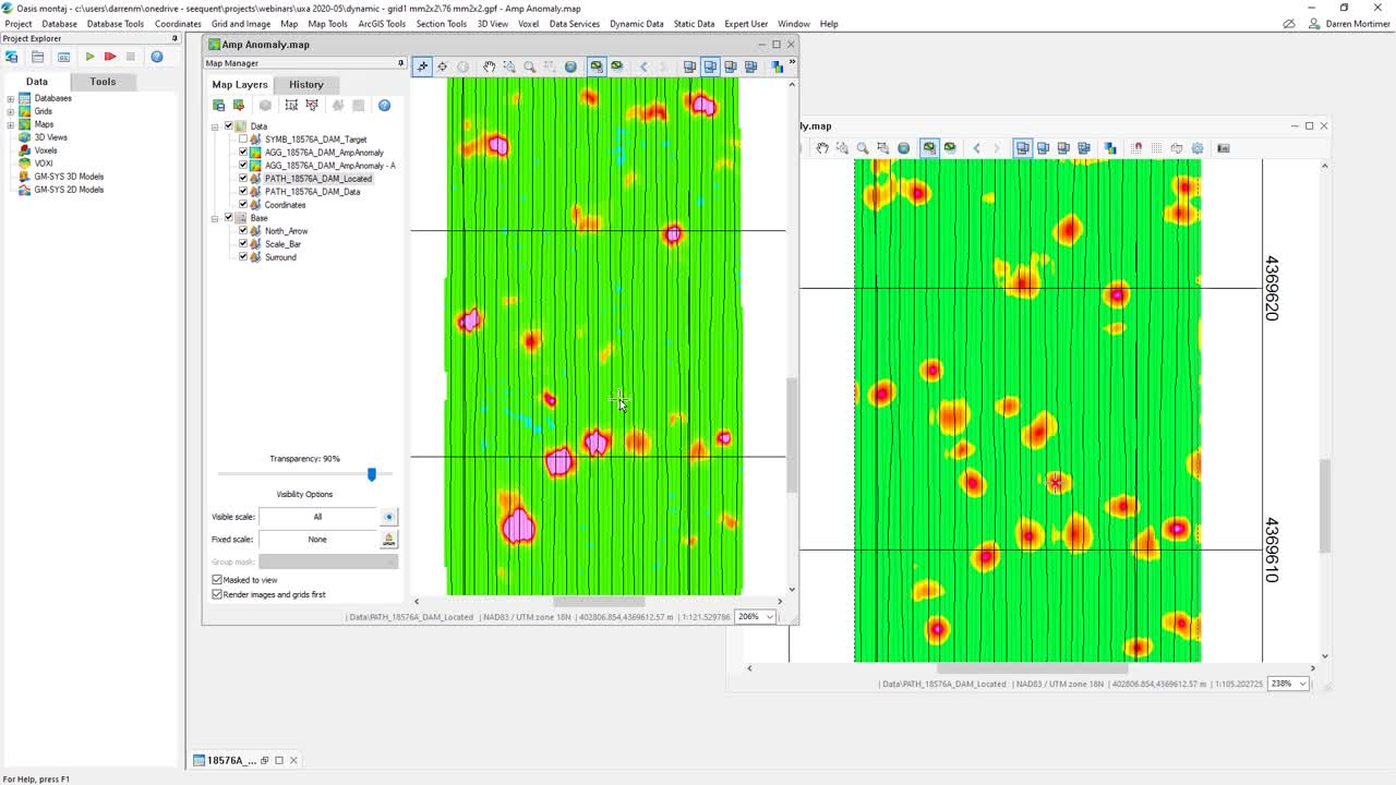
and shown it on here with our survey tracks.

[00:18:38.860]
One of the tips that I’d like to share with you,

[00:18:41.150]
often I like to see where was the data collected?

[00:18:44.960]
What you’re seeing there on that path there

[00:18:46.970]
is the original path of the cart of the sensor itself.

[00:18:52.100]
But remember it’s got in the case of this,

[00:18:54.320]
this is a two by two system, it’s got, as I was showing you,

[00:18:57.107]
those are the diagrams, those four receivers on those.

[00:19:00.320]
Well, where were those traveling?

[00:19:01.960]
And we can load and display those,

[00:19:04.210]
but whoa, that is just crazy.

[00:19:07.100]
I can’t see anything there.

[00:19:09.630]
One of my tips is set the transparency,

[00:19:14.020]
lower the transparency down of something of that

[00:19:16.560]
sort of other paths, where we can still see them.

[00:19:19.450]
We can still see where the original, the cart went

[00:19:23.070]
and then where those air receiver coils

[00:19:26.270]
traveled across our dataset.

[00:19:36.260]
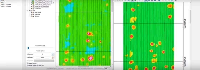
And one of the things that

[00:19:37.240]
once we’ve created this amplitude grid,

[00:19:41.530]
one of the other steps that we like to look at

[00:19:44.460]
is something we call the coherence anomaly.

[00:19:48.810]
And this is where we look at a sample of the data

[00:19:52.910]
and see how well an item will model

[00:19:58.180]
under a window of that data.

[00:20:00.170]
And I’ll show you some examples of the threshold plots

[00:20:04.630]
in a moment.

[00:20:08.240]
The coherence anomaly map, let’s just move this over here.

[00:20:13.480]
I have gone and created one.

[00:20:16.410]
It makes it very easy to detect targets which you may miss

[00:20:23.819]
in the amplitude plot.

[00:20:29.300]
Now maybe we’d like to see our line paths on here as well.

[00:20:32.540]
And since I’ve already created them

[00:20:34.820]
over on my amplitude map,

[00:20:37.120]
it’s as easy as just I can drag and drop them onto this map

[00:20:42.020]
and we can see them there.

[00:20:44.530]
And they’ll come across

[00:20:45.770]
with their same transparencies and everything that we have

[00:20:51.230]
on the previous map.

[00:20:53.510]
And don’t forget, if you’re looking to look at multiple maps

[00:20:58.850]
and gee, wouldn’t it be nice if they were at the same place.

[00:21:02.110]
At the top of the map there is a series of buttons.

[00:21:05.840]
If I click on the second button from the left,

[00:21:09.250]
that will make all my maps zoom to the same area

[00:21:13.040]
that I see on the map that I am controlling it from.

[00:21:20.760]
For those, if you have run that UX-Analyze before,

[00:21:25.050]
any of you have noticed areas where you might see this

[00:21:28.410]
or some of these like broad high features

[00:21:31.330]
in your coherence anomaly data?

[00:21:35.840]
This is generally caused by over-correcting your data

[00:21:40.550]
or over leveling your data.

[00:21:42.470]
When you’re doing the leveling,

[00:21:46.100]
look at going in and adjusting parameters,

[00:21:51.620]
the leveling of filtering the data

[00:21:53.710]
to changing perhaps your amplitude threshold

[00:21:57.520]
or the width of the signal

[00:22:00.100]
that you’re using to do the filtering.

[00:22:04.417]
It says those types of areas where you see the broad,

[00:22:09.196]
in the broad high in the coherence anomaly,

[00:22:13.070]
or perhaps a broad low in the amplitude

[00:22:16.410]
is an indication that you’ve over leveled

[00:22:18.870]
or over filtered your data.

[00:22:21.260]
And after I went through and adjusted that,

[00:22:25.790]
we can see how I can make those a little bit more clearer.

[00:22:35.840]
Now I mentioned earlier that the coherence anomaly

[00:22:38.420]
allows us to see anomalies which we might not

[00:22:43.250]
be readily see in the amplitude.

[00:22:46.470]
Here I’ve just got to made a match snapshot,

[00:22:48.057]
you know, if you send maps to your friends

[00:22:51.890]
or to your manager or senior scientists to have a look at

[00:22:57.020]
and review?

[00:22:58.270]
So here, if I want to send this map on,

[00:23:00.090]
I’ll say, Dave, look, there’s a spot here

[00:23:02.460]
where I’ve got these low amplitude anomalies

[00:23:04.280]
and they’re only coherence elements.

[00:23:05.640]
What do you think?

[00:23:07.330]
He’s like, you know, rather and he’s got to look at this data

[00:23:09.690]
and go, well, where does he Darren want me to look?

[00:23:13.160]
He can just come unload that snapshot

[00:23:16.590]
and it will go to that area

[00:23:18.190]
and if he turns on the changing stance on all maps,

[00:23:23.010]
you can now quite easily,

[00:23:25.560]
we can go on and turn on our shadow cursor

[00:23:27.600]
and see which of those anomalies

[00:23:29.800]
we can see quite clearly on the coherence map,

[00:23:34.440]
but not so much in just the amplitude or response alone.

[00:23:46.370]
We would go on after we’ve, can pick our anomalies

[00:23:50.370]
from both the coherence and the amplitude picks

[00:23:59.840]
and using the thresholding tools,

[00:24:02.300]
we can sort of decide which threshold we used.

[00:24:04.660]
In this data set I used 0.5 and three

[00:24:07.495]
and I’ll show you in a moment how I picked those

[00:24:11.200]
when I flipped back to the slides.

[00:24:13.730]
And finally, you will invert the data

[00:24:19.610]
and generate the sources and then you need to be to filter

[00:24:23.180]
and look at those sources

[00:24:27.520]
and determine which ones are something

[00:24:30.160]
that you would like to go on and go on to

[00:24:33.770]
and collect a static survey data.

[00:24:38.720]
And I had a, so I just took slow open up my source database

[00:24:43.410]
where I’ve gone and done this.

[00:24:50.980]
In the source database.

[00:24:56.320]
So we go from survey data, we pick targets,

[00:25:00.140]
we then invert those targets to generate sources.

[00:25:04.890]
And then we might learn to look at,

[00:25:07.150]
and I’ll just overwrite the one I made earlier

[00:25:09.540]
of being able to filter out some of the sources

[00:25:13.240]
because some of them may be things which just,

[00:25:17.330]
there’s no way that they can be the

[00:25:20.590]
type of target of interest or UXO that we’re looking for.

[00:25:24.650]
And to make this easier or to help you with that,

[00:25:27.100]
when you do the filtering step,

[00:25:29.260]
we create a bunch of channels and we look for

[00:25:33.940]
how big was the source?

[00:25:37.535]
Did we get a good inversion result?

[00:25:38.368]
If we didn’t get a good inversion result

[00:25:40.520]
because of noise or something in the data,

[00:25:42.630]
then we can’t trust that result.

[00:25:44.630]
And we want to keep that on our list

[00:25:47.158]
for further investigation.

[00:25:49.740]
Some things we might say,

[00:25:51.740]
well, look, there’s no way it could have a size and decay

[00:25:57.580]
that that could be something that we could

[00:26:00.050]
possibly classify.

[00:26:01.760]
And these then are indicated in one of the channels here,

[00:26:07.150]
they’re sort of flagged off of that.

[00:26:09.440]
And there’s a nice, clear channel that tells you

[00:26:13.510]
or a column in the data as to why they were filtered out.

[00:26:17.290]
And you can see those various symbols represented on this

[00:26:21.420]
feature space of scatter plot.

[00:26:24.570]
The red lines represent my thresholds for my size and decay.

[00:26:31.490]
So you can see symbols out there turned off or gray,

[00:26:36.560]
whether it be green and turned on in here,

[00:26:40.450]
some of them were found just to simply have no anomaly

[00:26:43.910]
like we had no signal

[00:26:45.940]
in that when we do some of the inversions,

[00:26:48.820]
we will look for what we call three dipoles, three objects.

[00:26:53.920]
And one of the dipoles will have an object.

[00:26:58.490]
One or two of the others may not

[00:27:00.860]
if there’s only one physical object there.

[00:27:04.720]
And those will be filtered out and removed.

[00:27:09.340]
Some of the ones you see here with a little brown Xs

[00:27:12.230]
or orange Xs all over the site and some just on the edge,

[00:27:17.620]
these are the ones that due to some noise in the data

[00:27:20.510]
that we had a poor inversion result.

[00:27:22.430]
And we want to keep a new ongoing revisit in our static survey

[00:27:26.980]
to make sure that there is no targets of interest there

[00:27:30.860]
’cause remember, we’re dealing with UXOs here,

[00:27:32.920]
we want to be conservative.

[00:27:36.360]
So there’s a little bit of a high-level overview

[00:27:38.830]
and a few tips on the dynamic processing.

[00:27:45.250]
And just flipping back to our slides here,

[00:27:47.950]
we kind of walked through some of that workflow,

[00:27:54.880]
and I promise you to looking at the coherence threshold

[00:28:00.790]
or how we pick those thresholds.

[00:28:03.000]
So there’s a tool called

[00:28:04.140]
determined coherence anomaly threshold

[00:28:06.450]
that creates this plot for you.

[00:28:10.480]
And one of the questions I often get asked is,

[00:28:14.070]
well, how many samples should we use when we do this tool?

[00:28:19.210]
And you can see there on the right

[00:28:20.420]
I’ve just kind of highlighted where that sample box is.

[00:28:24.880]
We generally recommend that people use around

[00:28:27.400]
about 2,000 samples.

[00:28:29.530]
And the question is, well, why do I need to use 2,000?

[00:28:33.060]
I want to get it done faster. I want to use less.

[00:28:37.030]
This example where I use just 20 points,

[00:28:44.190]
where we go and find a background area.

[00:28:47.340]
So an area that we believe

[00:28:49.240]
because of its signal is free of metallic debris.

[00:28:52.820]
We synthetically insert a signal response into that

[00:28:59.360]
and invert it and see how well that inversion goes.

[00:29:04.465]
If it’s a very good match to something,

[00:29:06.100]
that gives us a strong coherence.

[00:29:09.280]
And we can look at how noisy that is

[00:29:11.720]
compared to when we just try to invert it

[00:29:14.760]
when nothing’s there.

[00:29:17.020]
With the object, gives us the black dots.

[00:29:19.860]
Without the synthetic object there,

[00:29:21.990]
it gives us the red dots.

[00:29:24.680]
And there’s the thresholds that I picked before

[00:29:28.950]
in our example.

[00:29:32.200]
And you can see there’s with 20 points.

[00:29:33.610]
If I ran it another time with this 20 points,

[00:29:36.250]
because we randomly picked the locations,

[00:29:40.860]
you get a slightly different result.

[00:29:43.330]
So maybe 20 is not good enough.

[00:29:46.260]
So use 200.

[00:29:49.050]
It’s better,

[00:29:50.950]
but I run it with another 200 points.

[00:29:53.900]
Things will slow the shift again.

[00:29:57.450]
Yes, I did run a couple of examples

[00:29:59.550]
to run several runs to cherry pick,

[00:30:02.760]
to give you some examples where you could clearly see

[00:30:05.570]
the shifts occurring.

[00:30:09.120]
But if I ran it with 2,000 points,

[00:30:14.060]
all of those variations that you see do get covered in,

[00:30:17.390]
it gives you a much more reliable set of curves

[00:30:21.730]
to bid a pick from, making an awesome,

[00:30:24.640]
makes them very easy to interpret and see.

[00:30:31.610]
If you’re wondering why the two levels

[00:30:34.020]
on the coherence plot,

[00:30:37.299]
depending on the nature of your munition,

[00:30:42.760]
we can get this sort of down curve into the y-axis.

[00:30:46.830]
And I went and picked a sort of more conservative point.

[00:30:51.700]
The purple line is the depth of investigation

[00:30:55.660]
that we’re being asked for on this project.

[00:30:58.890]
Is we’ve been asked to find things like

[00:31:03.590]
a 37-millimeter or something that can also be represented

[00:31:07.000]
by a medium ISO down to 30 centimeters.

[00:31:10.850]
ISO stands for Industry Standard Object.

[00:31:14.620]
And so that’s the level I want to pick for.

[00:31:18.600]
I want to be maybe a little conservative

[00:31:20.510]
and that’s why I’ve gone and lowered my threshold

[00:31:23.490]
down to 0.5.

[00:31:25.770]
Yes, could I go lower?

[00:31:27.780]
But that would be going sort of above and beyond

[00:31:30.470]
what we were asked for in our project scope.

[00:31:39.890]
So now we’ve chosen our thresholds.

[00:31:42.270]
There’s two places that we use the thresholds.

[00:31:44.470]
And my other little tip is when you take your values

[00:31:48.530]
that you’ve used in your target picking,

[00:31:51.700]
I ended up typing in three I guess or could have used 3.7.

[00:31:55.320]
I think I had 3.6 sort of in around there.

[00:32:02.570]
Those are the values that we picked targets with.

[00:32:05.140]
When we do the inversion because we have this full coverage

[00:32:08.240]
that we get with dynamic data.

[00:32:10.630]
If a source is found to be on the edge of the data chip,

[00:32:15.340]
that piece of data that we use to do the inversion with,

[00:32:19.690]
our results aren’t going to be as good or as reliable.

[00:32:23.130]
But because we have that full coverage,

[00:32:25.000]
we can reposition that chip.

[00:32:29.960]
During that repositioning

[00:32:31.300]
we want to look to see if we’ve got data there

[00:32:34.080]
and it’s got some signal to it.

[00:32:36.230]
Like if it’s not gone into total background.

[00:32:41.100]
And we recommend there for your thresholds

[00:32:44.020]
that you use roughly about 50%

[00:32:46.130]
of the original target picking threshold.

[00:32:49.100]
But be careful, don’t go down into the noise.

[00:32:51.730]
If your site tends to be a little bit noisier

[00:32:53.670]
in your original target picking threshold

[00:32:56.040]
is close to a noise threshold,

[00:32:58.760]
you might not be able to actually go that full 50%

[00:33:02.460]
and we’ll need to modify that value.

[00:33:05.210]
But on hand, generally,

[00:33:06.720]
you can use 50% of your target picking threshold

[00:33:09.930]
for your repositioning threshold

[00:33:12.290]
when we’re doing the inversions.

[00:33:18.640]
So that’s a bit of a walkthrough

[00:33:19.990]
and some tips around the dynamic workflow.

[00:33:22.640]
Remember if you have any questions,

[00:33:24.170]
do enter them into the questions box

[00:33:25.860]
and we’ll respond to you after the webinar.

[00:33:32.200]
Next here, I’ll take a look at the static survey

[00:33:35.450]
or classification workflow.

[00:33:38.660]
For this workflow there’s really just two steps.

[00:33:41.910]
Prepare the data and classifying rank.

[00:33:45.260]
There is this step in the middle there,

[00:33:47.780]
construct and validate a site library.

[00:33:50.480]
This is something you generally just do at the beginning

[00:33:52.840]
or end of your project to make sure

[00:33:55.680]
that the library that you’re using

[00:33:57.410]
is a complete library for your site.

[00:34:01.670]
And we’ll come and look at that

[00:34:03.150]
notion of a complete library for your site

[00:34:05.090]
a couple points through this part of the presentation.

[00:34:10.310]
So here’s our a static workflow.

[00:34:12.950]
Much like my title that seemed to be,

[00:34:14.810]
today seem to be very long

[00:34:15.890]
and might look to be very complicated.

[00:34:18.090]
But again, I can sort of highlight for you

[00:34:20.810]
with the same closes on a general workflow.

[00:34:22.690]
Those must do points are shown there with those arrows.

[00:34:28.100]
And it’s really, you know, import some data, level it.

[00:34:33.180]
If it’s the first time through

[00:34:34.650]
and you haven’t got a library,

[00:34:39.241]
you should validate your library

[00:34:41.600]
and then it’s just classifying rank.

[00:34:43.340]
But for most of your project import level classify.

[00:34:50.480]
And it’s pretty much that simple.

[00:34:52.690]
So let’s go over to Oasis and I’ll show you just

[00:34:57.760]
exactly how simple that is.

[00:34:59.470]
I’ve created a project,

[00:35:01.290]
I’ve already imported my background data

[00:35:04.660]
and then now we will go in and import my survey data.

[00:35:14.470]
I’ll just turn off the filter here.

[00:35:16.910]
In this folder

[00:35:17.860]
I’ve got all of my different types of survey files.

[00:35:20.750]
We have SAM or static anomaly measurements.

[00:35:23.940]
We have other QC ones which I’ll touch on

[00:35:26.620]
a little bit later as QC sense of function tests.

[00:35:30.850]
And then my background measurements as it says,

[00:35:32.800]
I’ve already done those.

[00:35:34.650]
The import with the HDF import,

[00:35:38.400]
you can just give it all of your data

[00:35:41.270]
and we’ll figure it and put the data

[00:35:43.500]
into the right databases for you based on its data type.

[00:35:47.400]
I’ve just gone and selected for this demonstration here,

[00:35:50.700]
just for files, static anomaly measurements over some items.

[00:35:56.990]
So we can import those in.

[00:35:59.110]
You’ll get two databases.

[00:36:01.930]
A data database and a target database

[00:36:05.020]
and there’s a similar ones in the dynamic workflow.

[00:36:07.840]
The data database, tongue twister it is,

[00:36:10.660]
contains the actual transient or response data.

[00:36:13.940]
The target database contains this a list,

[00:36:17.470]
in this case of all the measurements that you made

[00:36:22.410]
and various sort of other parameters

[00:36:25.870]
of the sensor that was UBIT size windows,

[00:36:29.880]
other premises that we use that describe the sensor

[00:36:32.670]
that we then use in the inversion.

[00:36:36.400]
So once I brought it in, I need to level it.

[00:36:39.270]
Leveling it is removing the geology or background

[00:36:43.220]
or drift or the sensor out of the readings.

[00:36:49.950]
So we’re here.

[00:36:50.860]
I just need to pick my survey database

[00:36:54.780]
and my background database.

[00:36:57.090]
We find those based on the codes

[00:36:59.260]
that are there in those names.

[00:37:01.290]
And then we will just a couple options that we need to pick.

[00:37:05.550]
Most people will pick time and location.

[00:37:08.280]
You going to pick the nearest background reading

[00:37:12.110]
that was taken in an area that was free of metal objects

[00:37:17.220]
and subtract that from our measurement.

[00:37:21.030]
And we want to use the one that’s the closest in space,

[00:37:23.830]
most likely the same geology and the closest in time

[00:37:28.450]
to remove any drift.

[00:37:32.810]
And that will give us a new level channel.

[00:37:36.640]
And now we are ready to do our classifying rank.

[00:37:41.200]
I’ve already got a library. It’s a good library.

[00:37:44.520]
I’ve done my validate library work.

[00:37:46.200]
So I can just hit classifying rank.

[00:37:55.320]
We give it our database to use.

[00:37:59.920]
Is asking us what channels you may be using

[00:38:02.120]
as a mass channel.

[00:38:03.820]
A mass channel is a way that you can turn off

[00:38:06.700]
individual targets or flag or measurements and not use them.

[00:38:13.670]
So if you just wanted to do a sample or redo something,

[00:38:17.220]
this is a way that you could toggle that.

[00:38:20.520]
Some parameters about the sensor,

[00:38:24.930]
but the library database that we’re going to match to,

[00:38:27.690]
I can go onto the tools tab and these are all the individual

[00:38:31.100]
sort of steps that this tool

[00:38:35.020]
of classifying rank will go through.

[00:38:37.010]
We’ll invert your sources, do the library match skill,

[00:38:40.070]
look to see if there’s any self matches or clusters,

[00:38:43.900]
identify those and ultimately do that set the thresholds

[00:38:48.350]
and do our classification and prioritization.

[00:38:51.280]
We can also create several plots.

[00:38:54.540]
I’ll just do the one plot at the end of this to speed it up

[00:39:00.810]
for our demonstration today.

[00:39:05.630]
So there we go.

[00:39:06.463]
That’s going to take about two minutes to run

[00:39:11.820]
and just kind of go through all of those steps for us

[00:39:15.330]
and generate plots for each of those targets that

[00:39:21.215]
we read in.

[00:39:26.530]
But while that’s running,

[00:39:28.180]
we can just take a look at

[00:39:33.800]
a data set that I have already brought in,

[00:39:36.720]
much more targets and have ran through,

[00:39:44.910]
sorry, this one.

[00:39:48.750]
And this is after I’d ran my validate library workflow.

[00:39:54.110]
Is where this one is at.

[00:39:56.220]
And some tips of things that are good to look out on here.

[00:40:05.780]
We will load a series of channels, there’s lots of data

[00:40:09.330]
in the database table that you can look at.

[00:40:13.500]
That’s just my progress bar.

[00:40:15.350]
But two that are good to add and show here

[00:40:18.600]
are the ones that look for clusters.

[00:40:22.390]
So I can hit down our list,

[00:40:24.850]
drop down and there’s are two clusters, channels.

[00:40:30.911]
And you can see over in my plot

[00:40:32.840]
where you see a whole bunch of gray lines

[00:40:34.700]
on this one that I happened to be sitting on in behind.

[00:40:37.330]
And that’s the notion of a cluster that they are the same,

[00:40:41.480]
has the same set of polarizabilities.

[00:40:43.390]
In the EM sense, they look alike.

[00:40:48.420]
And during the validation stage,

[00:40:50.490]
you want to look for these unknown items and find those.

[00:40:53.540]
And one of the easy ways to do that

[00:40:56.480]
is to come to our tool here.

[00:41:01.950]
That just keeps popping up

[00:41:03.150]
and just do show a symbol profile.

[00:41:06.240]
And in your profile window, we’ll give you,

[00:41:11.410]
we create an ID for each of the unknown clusters

[00:41:15.430]
and in this window now we can sort of, you know, see those.

[00:41:20.000]
And so we can see this like three lines here if you would,

[00:41:24.700]
that these guys are all the same as this

[00:41:27.620]
’cause this is the ID for this cluster.

[00:41:30.110]
So is a cluster called number two.

[00:41:33.590]
And there’s a bunch of things that look like each other

[00:41:35.970]
that are in this cluster.

[00:41:37.880]
And I can flick between those.

[00:41:40.210]
I’m just going to move that to my second screen

[00:41:44.861]
and it will generate and bring up the plots for those.

[00:41:49.847]
And we can see, well, oops, didn’t click on it quite there.

[00:41:55.680]
There we go.

[00:41:56.513]
Click into the database and you can see it of those.

[00:41:59.420]
So as a time saving tip,

[00:42:02.170]
when you’re doing your validation of your library,

[00:42:09.770]
you can bring this up

[00:42:11.770]
and just do a simple plot of the cluster IDs

[00:42:15.990]
and see quite easily then any of the things

[00:42:19.050]
of the eye of the clusters that we can explain

[00:42:22.760]
in that they don’t have a strong match

[00:42:24.410]
to something in our library.

[00:42:27.380]
Maybe you want to look at, well, what did they match to?

[00:42:30.910]
And you could bring up one of the other plots

[00:42:32.700]
which I have shown up here in the top right.

[00:42:38.800]
But I could show those what they match to

[00:42:41.770]
and what the match metric,

[00:42:43.260]
how well those curves match to each other.

[00:42:46.300]
We come up with a quantitative value there.

[00:42:49.890]
I could load those,

[00:42:51.220]
but one of the key powers of using the tables,

[00:42:56.260]
because we have a lot of information

[00:42:57.890]
is to use the database views.

[00:43:01.270]
And I have gone prior to this and saved myself a view

[00:43:04.410]
that I would like to have and I can get that.

[00:43:07.640]
And just by simply coming in and loading my view,

[00:43:15.600]
I can do that same step that I did

[00:43:19.040]
and showed you manually a moment ago,

[00:43:20.940]
loading those cluster channels,

[00:43:22.930]
but I can also then go and load a whole bunch of

[00:43:26.440]
whatever other channels I would like to look at.

[00:43:28.980]
Here look where we’ve matched all three curves,

[00:43:33.530]
one, one, one.

[00:43:36.760]
Where we’ve just matched two of the curves are primary

[00:43:39.130]
and the secondary curve.

[00:43:41.810]
And what did they all match to.

[00:43:46.270]
From a real power user point of view

[00:43:48.170]
for you guys there that are advanced users,

[00:43:53.730]
these database of view files are text files.

[00:43:57.510]
You can go in and edit them.

[00:43:58.880]
There’s the one that I just loaded up.

[00:44:03.370]
When we run the bundles,

[00:44:04.800]
we give you an automatically load up a database view.

[00:44:10.380]
If you don’t like or continually want to add things

[00:44:14.250]
to the database view that we have,

[00:44:16.740]
you can go and edit that file.

[00:44:18.960]
And add your own channels that you would like to see

[00:44:22.370]
loaded in there.

[00:44:23.430]
And then every time you run classifying rank

[00:44:26.060]
or the validate library,

[00:44:29.040]
that series of channels will be loaded.

[00:44:36.310]
So at this point a moment ago, when we saw there was

[00:44:43.800]
progress priors stop are example that we did there.

[00:44:50.490]
We brought in in here has completed.

[00:44:52.890]
It’s found that those items match to

[00:44:56.470]
and we’ve got some pretty good match metrics.

[00:44:58.740]
And if I click on the item,

[00:45:01.910]
we will automatically bring up

[00:45:03.630]
and show us one of the plots.

[00:45:06.400]
And we can see the polarizabilities on here.

[00:45:11.670]
We can see the polarizabilities

[00:45:13.690]
and how well that they’ve matched.

[00:45:15.910]
We can see where the sensor was parked and laid out.

[00:45:19.330]
They parked really good,

[00:45:20.500]
right over top of the potential flag location

[00:45:25.010]
of where the source is

[00:45:26.080]
and it was found to be at that location.

[00:45:28.090]
And will show you some other plots

[00:45:29.480]
which I’ll come to in a moment.

[00:45:30.820]
There’s our size and decay friend again,

[00:45:33.000]
and this other one called the decision plot.

[00:45:37.180]
And I can just kind of go through and look at those.

[00:45:39.900]
This one didn’t match as quite as well.

[00:45:41.520]
You can see the polarizability is from our data

[00:45:43.987]
and this one with a little bit noisier,

[00:45:46.360]
and we didn’t get still matched to

[00:45:49.910]
a one 20-millimeter projectile,

[00:45:55.380]
but just compared to one of those first ones I looked at,

[00:45:58.160]
they were just a little bit more noisier.

[00:46:01.060]
And so you’d see that was just as easy as import data,

[00:46:05.270]
level it and run classifying rank.

[00:46:10.870]
When we want to come and look at our results,

[00:46:15.180]
that was the one we were looking at before.

[00:46:17.030]
Here’s where I have gone and ran a larger sample.

[00:46:21.820]
And you can see there’s our size and decay plot

[00:46:24.490]
that gives us that,

[00:46:25.670]
looking at that feature of those two properties

[00:46:28.420]
and where things might group.

[00:46:30.300]
They’re colored based on red, we think it’s a TOI,

[00:46:34.840]
target of interest.

[00:46:35.710]
Green, it’s a below some threshold that we set

[00:46:40.180]
of how well things match to library items.

[00:46:45.580]
And that’s shown here in a little,

[00:46:48.410]
what we call a decision plot.

[00:46:51.980]
We can bring other plots up

[00:46:56.330]
or any other images that you may have on

[00:46:58.500]
that you want to see in your data.

[00:47:00.600]
We can create what these plots

[00:47:03.100]
that we call interactive image of yours.

[00:47:05.500]
This could be any image that you have.

[00:47:07.601]
Some people like to do this when they do their dig surveys,

[00:47:11.440]
that they will use photographs of the items.

[00:47:15.150]
And creating a view as simply as looking at the images

[00:47:23.080]
that you’ve created.

[00:47:23.913]
So this is my folder of some images that I,

[00:47:28.780]
polarization plots that I created earlier.

[00:47:31.970]
Seeing what the name is there and generally

[00:47:34.370]
we’ve got everything there with a prefix.

[00:47:36.590]
And then the name of the item is the last part of that.

[00:47:43.580]
And in this case that name is referring to

[00:47:49.070]
its initial acquisition ID.

[00:47:52.290]
So I’m going to go find that in the list here

[00:47:57.370]
and then browse into that folder.

[00:48:04.780]
And we’ll look in that folder and try to figure out

[00:48:07.030]
whether you’ve got a prefix as in my case, or,

[00:48:10.087]
you know, maybe you’ve done a suffix on there

[00:48:15.090]
for naming all the images and then whether the PNG, bitmap,

[00:48:22.350]
JPEG, whatever and then you can load it.

[00:48:30.272]
And then when I click on any one of our sources,

[00:48:35.030]
that image will load up along with my other image.

[00:48:38.010]
I can see here and we can look at it

[00:48:41.120]
and help you do the review.

[00:48:43.060]
Now, maybe you’re like me,

[00:48:44.520]
and you’ve got all these over and you’d be like,

[00:48:46.320]
gee, it would be nice if I could get them to arrange

[00:48:50.310]
the way that I would like them to arrange.

[00:48:54.440]
And for that, you could go,

[00:48:56.100]
we have a tool that will let you save a window layout.

[00:48:58.960]
Earlier I saved a window layout

[00:49:01.980]
and I had one from a self to get started,

[00:49:05.200]
but then I also had one for my classifying rank.

[00:49:07.620]
So I can load that one.

[00:49:09.690]
Oh, wait.

[00:49:10.900]
Sorry, I clicked on the wrong button there.

[00:49:27.290]
So is easy as that.

[00:49:29.150]
Now my window’s all arranged

[00:49:31.480]
in a way that I would like them to be

[00:49:34.800]
and I can easily move through

[00:49:37.140]
and they will update as I go forward and look at the plots.

[00:49:43.030]
We also have other tools.

[00:49:44.710]
I have a size and decay plot on that

[00:49:48.326]
main documentation plot that I made,

[00:49:51.560]
but maybe I would like to have an interactive version

[00:49:55.540]
of one of those so that when I click on it,

[00:49:58.840]
things will change and we can open up

[00:50:01.210]
and create one of those.

[00:50:06.860]
You can load overlays onto these plots

[00:50:10.760]
to help you find some of the items

[00:50:13.580]
that you were looking for.

[00:50:14.570]
And I’ve made an overlay earlier.

[00:50:22.100]
You can color them up based on one of the parameters.

[00:50:27.340]
If you do that based on the category,

[00:50:30.120]
we’ve got already a color code pattern in there

[00:50:32.950]
that will load.

[00:50:35.940]
So you can use that and this is always interactive

[00:50:38.770]
so that when I click on one of these items,

[00:50:41.910]
on the scatter plot, my database will go to it.

[00:50:45.920]
And as long with the other plots

[00:50:47.680]
that I am looking at and reviewing.

[00:50:54.620]
So there’s just a little bit of a walkthrough.

[00:50:59.590]
And I’m looking at some features with the static workflow.

[00:51:05.530]
And I’ll just kind of, you know, go back to my slides here.

[00:51:10.220]
And there was a couple of other,

[00:51:11.957]
you could say, frequently asked questions

[00:51:13.880]
I get from people, how to create a library.

[00:51:18.330]
Well, the answer’s real simple.

[00:51:20.940]
Collect some data over a target of interest.

[00:51:25.580]
With UX-Analyze we include an example library,

[00:51:30.270]
and this is based off a assertive ESTC project.

[00:51:34.760]
And I’ve included the link there

[00:51:36.790]
if you’d like to know about it.

[00:51:38.180]
But you can see some examples from that project where

[00:51:40.840]
they just took a sensor.

[00:51:42.210]
In this case, a MetalMapper,

[00:51:43.820]
put it on some plastic book stands

[00:51:48.690]
and then placed items underneath it and collected some data

[00:51:52.520]
that we then use as part of our libraries.

[00:51:57.997]
And as I touched on it in the demonstration.

[00:52:01.070]
Well, once these unknown items that are not on my site,

[00:52:05.953]
sorry, are not in my library, that are on my site.

[00:52:09.290]
Part of the validate library tool

[00:52:11.140]
looks for clusters of similar items

[00:52:14.870]
and then identifies the ones for you

[00:52:16.970]
which we don’t have an explanation for

[00:52:20.360]
that not in our library.

[00:52:22.290]
Then it’s up to you to go out,

[00:52:23.680]
collect some ground truth.

[00:52:25.570]
We identify which one is the most similar.

[00:52:29.735]
If you’re going to dig any of them up,

[00:52:30.800]
at least dig that one up.

[00:52:32.850]
Figure out what it is

[00:52:34.280]
and then there’s a tool where we can

[00:52:35.607]
add the item to our library as either a target of interest

[00:52:39.600]
or not a target of interest.

[00:52:41.830]
And then it will be used in the classifications

[00:52:43.780]
appropriately.

[00:52:48.390]
We have a number of quality control tests

[00:52:51.720]
because we want to make sure that the data

[00:52:53.183]
that we base our classification decisions on

[00:52:56.240]
is of the highest quality possible.

[00:52:58.710]
You don’t have time to go into those today,

[00:53:00.860]
but these have been developed to prevent common issues

[00:53:04.870]
and have all come from user feedback.

[00:53:08.500]
And there’s some,

[00:53:10.020]
it says those are the three main ones there.

[00:53:15.980]
How do we know this stuff works?

[00:53:18.470]
Oh, wait, sorry.

[00:53:21.680]
Reporting.

[00:53:23.690]
As you saw there,

[00:53:25.640]
the database tables can be easily exported out of

[00:53:29.010]
Oasis Montaj and then used in your reports.

[00:53:33.090]
All the plots that we generate are also saved as PNG files

[00:53:37.203]
so that you can then easily print them off,

[00:53:40.170]
include them in an appendix if you want to do that

[00:53:43.845]
and to share them among project stakeholders.

[00:53:51.180]
So how do we know that these things work?

[00:53:53.900]
Well we can look at something called

[00:53:55.330]
a receiver operating characteristic curves.

[00:53:58.870]
For a number of the demonstration projects of being done

[00:54:01.970]
while testing this types of technology.

[00:54:04.340]
They went and dug up all the items on the site

[00:54:07.290]
to see how successful the classification was.

[00:54:11.310]
So just there,

[00:54:12.670]
we have a sort of schematic of a rank dig list.

[00:54:16.570]
Red items are high confidence TOI,

[00:54:21.970]
yellow, most likely TOI and go on and dig them up

[00:54:25.590]
and then green high confidence none TOI.

[00:54:29.070]
Perfect classification, we would see a nice L

[00:54:31.700]
as shown on the left there or in the middle.

[00:54:34.640]
And if we just did a random guess 50, 50 guess,

[00:54:38.350]
you’d get something like a 45-degree line

[00:54:42.700]
on a one of these plots.

[00:54:46.350]
There is a tool in UX-Analyze.

[00:54:48.910]
If you want to do this to help calculate or create these

[00:54:53.050]
receiver operating characteristic or rock curves.

[00:54:57.765]
And from a couple of examples of the demonstration projects.

[00:55:01.560]
You can see, not quite at that sort of,

[00:55:04.330]
you know, perfect L-shape, but we’re pretty close

[00:55:09.400]
on some of them.

[00:55:10.850]
Some of these don’t go through zero by the way,

[00:55:13.150]
is because they asked for examples.

[00:55:15.390]
I hear they went and dug up some items to help them learn

[00:55:22.150]
or train the classification system.

[00:55:26.330]
So that’s how we know that we can reliably go and detect

[00:55:31.870]
and classify munitions or targets of interest

[00:55:36.130]
based on a geophysical response.

[00:55:41.550]
So in summary, today we’ve taken a look at

[00:55:43.042]
what is Advanced Geophysical Classification,

[00:55:46.670]
how we can use the EM response

[00:55:48.490]
to determine intrinsic property of the source,

[00:55:50.963]
the polarizabilities.

[00:55:52.277]
And those polarizabilities can be used for classification,

[00:55:56.480]
both whether it’s just a simple

[00:55:58.110]
matching to a physical property,

[00:56:00.070]
like size, shape, wall thickness.

[00:56:02.330]
Or actually using the signature mapping.

[00:56:06.150]
At the beginning there we saw how using

[00:56:08.730]
a method of classification

[00:56:11.480]
and being able to eliminate the clutter items.

[00:56:13.700]
We could reduce our excavation costs

[00:56:16.460]
and saving time and money on our projects.

[00:56:20.730]
We took a little bit of a look at dynamic

[00:56:24.290]
using dynamic advanced EM data

[00:56:28.544]
that gives you an improved target detection

[00:56:29.790]
and positioning over the conventional sensors

[00:56:31.860]
but you can use conventional sensors for the dynamic phase

[00:56:37.040]
is perfectly okay.

[00:56:39.840]
You’ll find you just have a few more re-shorts

[00:56:42.160]
when you’re doing your static classification survey.

[00:56:46.010]
And it’s possible with the static survey data

[00:56:50.020]
to reliably classify sources of geophysical anomalies

[00:56:53.340]
whether it’s a target of interest or not.

[00:57:01.120]
If you’d like to learn more about

[00:57:02.590]
Advanced Geophysical Classification,

[00:57:04.310]
we’ve got a couple online resources for you.

[00:57:09.308]
Going to their, there’s some papers and other presentations

[00:57:13.150]
that we’ve done and other examples.

[00:57:16.680]
If you’d like training, contact your local office,

[00:57:19.810]
so we can do remote training these days

[00:57:22.290]
or at some point set up a in-person training.

[00:57:26.710]
There is some material online

[00:57:29.430]
where you can go and also register for

[00:57:31.760]
some of our other training sessions.

[00:57:34.720]
Of course there is our support line

[00:57:37.780]
which you can read through a direct email

[00:57:39.600]
or through our website.

[00:57:41.130]
So hopefully you found this interesting and useful,

[00:57:44.510]
and I’d like to thank you for your time today.

[00:57:49.270]
And there’s my email again if you didn’t catch it earlier,

[00:57:53.070]
and thanks for your time

[00:57:55.650]
and hope you have a nice day.