Geological modeling with drillholes + What’s new in Geo (Remote Roundup 2021)

Geological units to be modeled include an erosional surface, a vein system, and 2 diorite intrusions. Wrap up the demo with a tour of the newest features in Leapfrog Geo.

Overview

Video Transcript

[00:00:00.000]
(moderate ambient music)

[00:00:11.110]
<v Anna>So if you didn’t know already,</v>

[00:00:12.750]
you are here for a demonstration of Leapfrog Geo,

[00:00:17.160]
this is going to be geared

[00:00:18.570]
toward those who haven’t seen Leapfrog Geo before,

[00:00:21.810]
or just need a bit of a refresher.

[00:00:23.570]
So we’ll be focusing on just building a model.

[00:00:26.140]
We’ll also do a little bit of data importing,

[00:00:29.280]
and then I also want to just chat casually

[00:00:31.620]
about some of the new features.

[00:00:34.850]
So hello again, my name is Anna Kutkiewicz.

[00:00:38.300]
I’m a senior project geologist with Seequent.

[00:00:41.030]
I’ve been with Seequent for about four years.

[00:00:43.110]
I started out on the development team in New Zealand.

[00:00:49.740]
Enough about me.

[00:00:50.573]
I don’t really want to spend too much time

[00:00:51.950]
about talking about myself.

[00:00:54.850]
We’ve only got a quick timeframe to go over everything here.

[00:00:58.550]
So I’m going to launch right in.

[00:01:01.160]
What is Leapfrog Geo?

[00:01:03.820]
Leapfrog Geo is a workflow based,

[00:01:06.020]
3D-implicit geological modeling tool.

[00:01:09.120]
It allows you to really quickly construct models

[00:01:12.390]
directly from various sources.

[00:01:13.980]
So that includes your drill holes,

[00:01:15.110]
but that also includes structural data points,

[00:01:18.670]
GIS data surfaces, and it uses something called fast RBF

[00:01:23.970]
which is a volumetric metric algorithm

[00:01:25.950]
that’s really good for constructing surfaces really quickly

[00:01:30.490]
based on data that might be really dense in one area

[00:01:33.260]
and really sparse in another area.

[00:01:36.090]
And then of course, because it’s implicit,

[00:01:38.230]
your models can be dynamically updated

[00:01:40.330]
to honor any new input data that you bring in.

[00:01:49.610]
Just a bit of a comparison,

[00:01:50.920]
we always like to compare it to some of those other ways

[00:01:55.650]
that can be a little bit more time consuming.

[00:01:57.890]
So Leapfrog, I’ve mentioned that it’s implicit,

[00:02:00.520]
so that compares to explicit,

[00:02:03.100]
which I’ve got a little picture down here.

[00:02:04.610]
So explicit is going to be drawing

[00:02:07.700]
all those painstaking polygons around your data in slice,

[00:02:14.150]
and then connecting them all together

[00:02:15.560]
with the triangulation.

[00:02:16.520]
So that can take a lot of time.

[00:02:18.330]
It’s really hard to bring in all of your drill holes,

[00:02:22.710]
your geology, your alteration, your weathering,

[00:02:27.170]
your structure, any mapping.

[00:02:28.620]
It’s just very difficult to bring all that on

[00:02:30.700]
into the same screen and try and create an interpretation.

[00:02:35.090]
Takes a lot of time to build or to update with new data.

[00:02:39.650]
And I think more importantly,

[00:02:40.590]
your interpretations and modeling are subjective.

[00:02:43.160]
So, I’m joined here by a colleague, Sarah Connolly.

[00:02:47.620]
She’s going to be taking questions at the end

[00:02:49.010]
if there are any,

[00:02:49.900]
but we might have the exact same background,

[00:02:52.370]
exact same training, exact same experience,

[00:02:55.410]
and still create two different models

[00:02:59.220]
using an explicit approach.

[00:03:02.770]
So on the flip side, implicit modeling,

[00:03:05.130]
we are basing the model on a continuous 3D function

[00:03:07.870]
to honor spatial data points.

[00:03:09.220]
So I guess point here,

[00:03:10.950]
you’re not making your interpretations

[00:03:12.440]
on strict slice across a given orientation.

[00:03:16.800]
It’s really easy to develop some type of bias

[00:03:20.260]
if you’re slicing continuously along the same orientation.

[00:03:23.720]
You might completely miss a trend.

[00:03:25.310]
I think we’ve all seen images or studies

[00:03:28.530]
where two geologists will have three different opinions

[00:03:33.680]
and especially if you’re only looking at the data

[00:03:36.070]
from one angle, it can be dangerous, I’ll say.

[00:03:42.370]
In Leapfrog, it’s really easy to incorporate

[00:03:44.130]
all of your data, that includes maps and sections,

[00:03:47.330]
and you can easily efficiently

[00:03:49.000]
update your models with new data.

[00:03:52.670]
Modeling is objective, so all those settings,

[00:03:55.560]
they’re easily reviewed.

[00:03:59.170]
So it’s very easy for two different people

[00:04:01.440]
with the same background to make a similar model.

[00:04:08.130]
Okay, so enough of the boring PowerPoint,

[00:04:10.540]
I’m going to go ahead and flip over to Leapfrog Geo.

[00:04:17.230]
When I’m giving a demonstration,

[00:04:18.350]
I like to show the finished product here.

[00:04:20.010]
So we’re looking at a 3D view

[00:04:21.830]
of our completed geological model.

[00:04:24.950]
So these volumes have volumetric information.

[00:04:28.730]
It is a water-tight model.

[00:04:30.350]
This one happens to be built directly from drill holes.

[00:04:33.560]
So I can just turn off a couple of these,

[00:04:35.000]
maybe give you a bit more of a preview

[00:04:36.460]
of what’s going on here.

[00:04:38.700]
So I’ve got some cross cutting day site dykes,

[00:04:42.730]
I’ve got an early diorite intrusion,

[00:04:44.810]
I’ve got an inner mineral diorite intrusion

[00:04:46.630]
then I’ve got this basement unit.

[00:04:49.430]
Now all of those surfaces are,

[00:04:51.370]
all of those volumes are guided by drill hole data.

[00:04:55.370]
So the way that it works is that it extracts points data

[00:04:58.530]
from contexts that you assign,

[00:05:00.770]
and then it constructs those surfaces from the points.

[00:05:03.180]
And you can further on edit those surfaces

[00:05:05.040]
with any data that you have.

[00:05:09.790]
Something to quickly point out here

[00:05:11.500]
is that the interface is really clean and uncluttered,

[00:05:14.550]
not a whole lot in the tool bar along the top here.

[00:05:17.570]
And that’s just because all the functionality

[00:05:19.410]
is located in what we call the project tree

[00:05:21.220]
on the left-hand side.

[00:05:23.590]
So if you start clicking on things,

[00:05:25.190]
you’ll see that there’s import options,

[00:05:26.860]
there’s generation options.

[00:05:28.340]
And this is also where all of your data lives.

[00:05:30.650]
So my geological model, my points, my drill holes,

[00:05:35.280]
and it’s all organized in a nice, clean,

[00:05:38.810]
workflow-based manner.

[00:05:43.010]
So to show you actually how this works,

[00:05:45.760]
I’m just going to go open a brand-new project

[00:05:49.700]
that has nothing in it.

[00:05:51.240]
I am going to be using something called Central.

[00:05:54.450]
This is your cloud-hosted project management system.

[00:06:00.390]
It has a lot of features,

[00:06:01.430]
I can’t even state them all in one sentence.

[00:06:03.550]
So if you’re curious about Central,

[00:06:05.090]
check out the demo on Wednesday at 3:00 P.M.

[00:06:09.610]
So this is one single project in Leapfrog.

[00:06:11.850]
I’m just going to go back in time

[00:06:14.040]
to the initial stage of the project

[00:06:18.930]
where there was nothing actually in it.

[00:06:20.310]
So if you look at my project tree here, it’s just empty.

[00:06:25.910]
Okay, so I’ll start with an easy import.

[00:06:27.650]
I’m just going to import points.

[00:06:28.930]
Again, I’m using Central,

[00:06:30.040]
so all of my data has been uploaded into my data room.

[00:06:34.600]
You can look at that later on Wednesday.

[00:06:39.750]
I’m going to navigate through my data room,

[00:06:41.780]
find my typography points and hit import.

[00:06:50.020]
Here’s a little preview of what the import will look like.

[00:06:53.260]
X, Y, Z, hit finish, that’s going to bring in

[00:06:56.020]
all of these points and I can load them in

[00:06:57.670]
and see what they look like.

[00:06:59.890]
Kind of a dynamic topography here.

[00:07:03.230]
I’m also going to show you the first example

[00:07:06.450]
of how Leapfrog generates circuses.

[00:07:08.770]
So I’m just going to make a new topographic surface

[00:07:11.690]
from points, select my points here, just call it topography.

[00:07:21.050]
And in Leapfrog, we’re using interpolation.

[00:07:24.220]
So I’m constructing a surface with a bunch of triangles,

[00:07:27.870]
very easy to go in and say,

[00:07:29.417]
“I want to make some finer triangles here

[00:07:31.650]
to get more detail in that surface.”

[00:07:33.850]
I’m just going to update that quickly

[00:07:36.680]
and then show you here’s my resulting surface.

[00:07:40.830]
If I just turn my point data off,

[00:07:42.360]
you can see how quickly that generated

[00:07:45.880]
a nice, reasonable surface.

[00:07:51.790]
Okay, so next set of data, I’m going to bring in drill holes

[00:07:56.160]
importing my drill holes via Central.

[00:07:57.720]
That is a new feature

[00:07:58.590]
for all of those existing Leapfrog users.

[00:08:01.650]
So, I’m going to grab my Wolf pass project

[00:08:04.610]
and go into the color, drill holes in topography.

[00:08:08.810]
I’m just going to grab the collar

[00:08:10.490]
and it should grab the other files.

[00:08:14.010]
It grabbed my survey.

[00:08:16.110]
So I’m just going to bring in my same recology,

[00:08:20.450]
hit import and then we’re going to get that importer wizard

[00:08:26.240]
designed to show you what types of data

[00:08:30.710]
you’re going to need to bring in,

[00:08:31.690]
but then it also does intelligently pick your aliases.

[00:08:34.450]
So whole ID, X, Y Z, next step I can just hit next

[00:08:37.890]
and go to the next table.

[00:08:41.040]
Survey looks all good.

[00:08:43.960]
So here’s my assay table.

[00:08:46.040]
I’m going to bring up my copper.

[00:08:48.670]
I’m going to bring in my gold and then finally my lithology,

[00:08:55.320]
that’s already going to come in as a lithology,

[00:08:58.200]
so hit finish.

[00:09:06.017]
Okay, so I’m just going to grab my lithology table here.

[00:09:10.430]
I’ll turn off the topography,

[00:09:12.320]
maybe turn off the points as well.

[00:09:15.200]
Make these a little bit easier to see.

[00:09:17.650]
So here I have my drilling.

[00:09:20.020]
I’m just going to turn on my legend.

[00:09:21.570]
So this is a pretty clean dataset,

[00:09:23.760]
but one of my favorite features in Leapfrog

[00:09:26.250]
is the ability to edit or make those interpretations

[00:09:30.680]
for modeling on the fly.

[00:09:33.070]
But we all know that there’s fields of lumpers

[00:09:36.750]
and splitters the core logger versus

[00:09:40.110]
when it actually gets to the geologist on the computer.

[00:09:44.110]
So that’s one of the things that you can do in Leapfrog

[00:09:46.187]
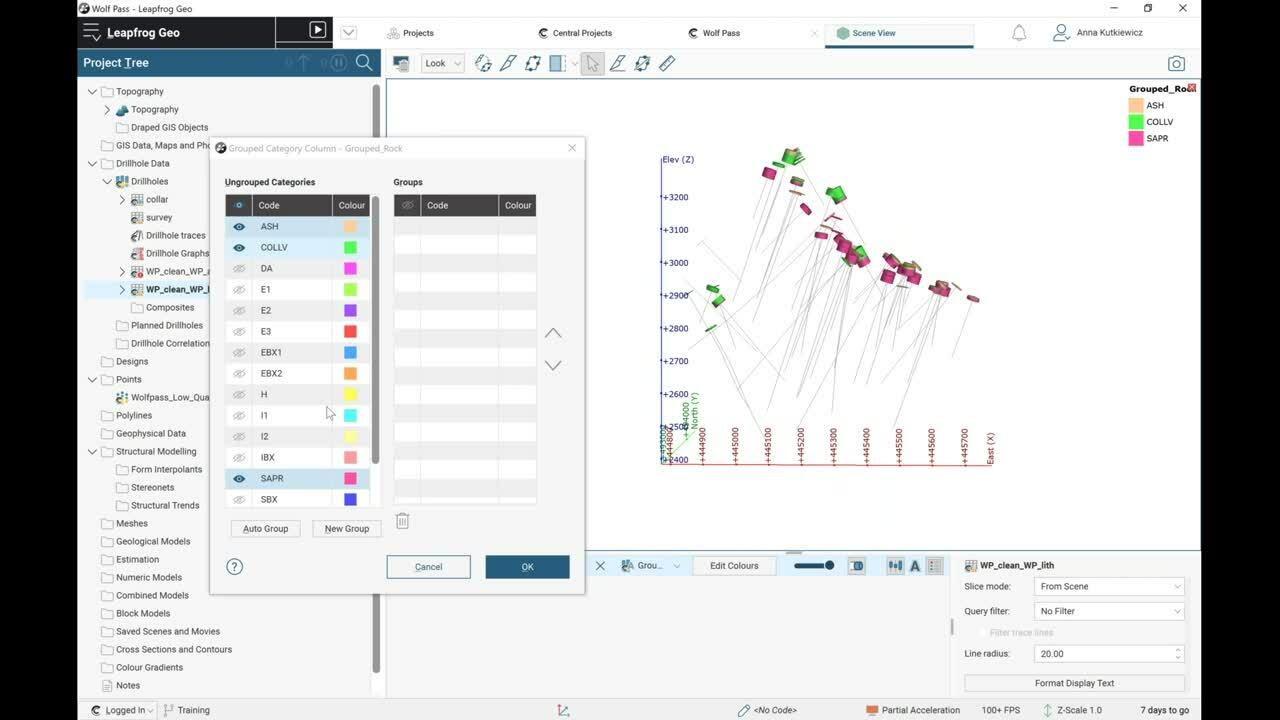
and we call it grouping.

[00:09:47.830]
And you’re never overwriting any of your data,

[00:09:49.630]
you’re just making a new column.

[00:09:51.690]
I’m going to group my lithologies, call it grouped rock.

[00:09:58.200]
So it’s like I’m adding a brand new column

[00:09:59.820]
on a table in Excel.

[00:10:02.440]
This is also organized to make it easier for us

[00:10:06.010]
to group things together.

[00:10:07.730]
So I’ll just turn them all off

[00:10:08.840]
and maybe I know that I want to group my Ash collutorium

[00:10:12.680]
and say my saprolite.

[00:10:14.120]
I think those are all hanging together

[00:10:15.650]
pretty well on the surface.

[00:10:17.260]
So I’m just going to grab those three and hit new group.

[00:10:19.870]
We’ll call that recent.

[00:10:23.960]
And I just moved through the rest of my data as well.

[00:10:25.900]
So maybe I want to group all of these in units

[00:10:31.240]
and I can always go back and later on refine that,

[00:10:34.730]
but maybe when I’m just starting out my interpretation,

[00:10:38.620]
I want to lump these to make my initial modeling

[00:10:41.690]
more easier to tackle from the get-go.

[00:10:46.830]
I’ll say in my eyes,

[00:10:50.040]
that’s going to be inner mineral diorite, we’ll see.

[00:10:55.492]
IM diorite,

[00:11:01.470]
and now I’ve got a basement shift unit.

[00:11:04.110]
I think I’ll just group those together in a basement.

[00:11:15.150]
And lastly, I’ve got this day site unit.

[00:11:17.240]
I’m still going to bring it over

[00:11:20.010]
so that it exists in that column.

[00:11:24.310]
And there we go, we have our new groups.

[00:11:31.120]
So if I just open up that table, you can see that I’ve not,

[00:11:34.080]
again, I’m not overriding anything,

[00:11:35.560]
I’ve just created this brand new grouped code.

[00:11:38.410]
I did ignore a unit called core loss

[00:11:40.300]
and I don’t want to model that.

[00:11:44.267]
Okay, so let’s look at the opposite situation,

[00:11:46.140]
another excellent feature in Leapfrog,

[00:11:48.750]
this might be the bread and butter selection.

[00:11:51.170]
So I’ve got this day site unit

[00:11:52.620]
and of course, when you’re logging this,

[00:11:54.710]
core log is not going to split it up

[00:11:55.900]
into different day site units or different courts.

[00:11:58.710]
That’s something that’s going to happen

[00:12:01.150]
in the modeling process.

[00:12:03.320]
In Leapfrog, it’s very easy to do that

[00:12:06.300]
with this tool called interval selection.

[00:12:09.720]
It’s called a selection.

[00:12:11.020]
I’m going to base this on my grouped field that I just made.

[00:12:17.450]
I’ve got more tools at the top

[00:12:19.257]
just because they’re only a couple to start.

[00:12:22.230]
You’ll notice that in other editors

[00:12:23.780]
there are further tools that will pop up.

[00:12:26.400]
So I’m just going to use my selection

[00:12:28.310]
and it works like a paint with a stroke.

[00:12:32.610]
Just grab some of those, maybe assign that to you

[00:12:34.700]
and I’ll just call this day site one.

[00:12:39.550]
I’m just going to rotate to make sure

[00:12:40.903]
that that makes 3D sense.

[00:12:43.240]
Yeah, okay.

[00:12:44.073]
So then I’ll grab those guys

[00:12:51.940]
and I’ll call that day site two.

[00:12:58.360]
Let’s make these colors a little bit more obvious,

[00:13:07.060]
and then save, just close that out.

[00:13:09.430]
So again, I’ve created yet another column on this table.

[00:13:12.270]
so it’s really easy to make interpretations

[00:13:14.273]
right in the program.

[00:13:16.700]
And I’m at the stage where this column is the cleanest.

[00:13:19.390]
I’m actually ready to go ahead and create my model.

[00:13:22.530]
That’s where I’m going to head to now.

[00:13:25.720]
Go into my geological models folder,

[00:13:28.030]
just create a new one,

[00:13:29.670]
choose the lift field that I want to use,

[00:13:33.810]
make the boundary of that a little bit smaller.

[00:13:36.110]
I’m just going to close my lithology.

[00:13:39.660]
I’m also going to set my triangle size and there we go.

[00:13:46.760]
So right now it’s just building the framework

[00:13:48.625]
of a geological model.

[00:13:50.230]
So it’s constructing a boundary,

[00:13:52.960]
it’s linking my lithology to my drill hole table

[00:13:56.110]
and actually want to point out.

[00:13:57.160]
So I’ve mentioned, or I mentioned in the intro

[00:13:59.740]
that Leapfrog is dynamic.

[00:14:00.950]
So that means that things within your project

[00:14:03.500]
are linked to other things.

[00:14:04.860]
So you’ll actually see that with a hyperlink.

[00:14:07.100]
So if I point out this selection here and if I click on it,

[00:14:10.653]
it’s going to take me exactly to that area in the project tree.

[00:14:13.950]
So that becomes very useful

[00:14:15.150]
when you’re generating your models,

[00:14:17.460]
you can actually see how things were built exactly.

[00:14:20.590]
Very easy to audit, again.

[00:14:25.800]
All right, so if I look back at all of my units here,

[00:14:30.760]
this color scheme isn’t awesome.

[00:14:34.650]
There we go, let’s make that a little bit brighter

[00:14:37.210]
and the way that Leapfrog works

[00:14:39.260]
is that it essentially starts out with this boundary.

[00:14:42.090]
So it’s already clipped by topographies conveniently,

[00:14:46.237]
and then you can build enclosing surfaces

[00:14:50.270]
around your geological units

[00:14:52.330]
and then they slice into each other.

[00:14:54.180]
So I’m just going to show you that process, easier to show.

[00:14:58.810]
So let’s just start with one.

[00:15:00.990]
I think since we just looked at our day sites,

[00:15:03.320]
I’ll start there and based on the geometry,

[00:15:08.090]
that’s how you can determine the different tool

[00:15:09.900]
that you’ll use in Leapfrog.

[00:15:11.390]
So this one indicates a vein system tool.

[00:15:13.990]
It allows you to say, I’ve got multiple veins within,

[00:15:18.750]
they’re all logged at the same lithology,

[00:15:21.030]
but maybe I want them to interact with each other.

[00:15:23.140]
I can say new vein, make a new vein from day site one.

[00:15:30.479]
I can see that that’s building.

[00:15:33.330]
And actually, while that’s processing,

[00:15:34.620]
I’ll mention that in Leapfrog,

[00:15:36.270]
you can always see what’s processing.

[00:15:38.100]
That was too fast.

[00:15:40.670]
If you’re impatient like I am,

[00:15:42.130]
that’s a really useful feature.

[00:15:44.040]
So if I’m creating another one here,

[00:15:46.370]
I’ll say on day site two, click okay.

[00:15:48.400]
I can always go into this processing panel.

[00:15:50.770]
See exactly what’s happening at the moment.

[00:15:52.880]
I can also pause.

[00:15:54.630]
You have a lot of flexibility

[00:15:55.820]
to see what’s actually going on.

[00:16:00.470]
Oh, I didn’t even show you day site one,

[00:16:01.940]
sorry about that.

[00:16:02.773]
Okay, so here’s day site one.

[00:16:04.390]
It is taking the hanging wall points

[00:16:07.250]
and it is interpolating a surface between those

[00:16:09.710]
and it’s doing the same thing between the foot wall points.

[00:16:13.030]
So if I now show you day site two, here we go

[00:16:19.970]
again, these colors are editable.

[00:16:22.020]
They do get automatically selected,

[00:16:23.772]
randomly selected as a start.

[00:16:25.950]
So here’s a case where

[00:16:28.140]
maybe I do want to set some type of interaction.

[00:16:30.390]
I want day site two to terminate against day site one.

[00:16:33.750]
That’s an option as well.

[00:16:35.490]
So within the vein system, I can say my day site two,

[00:16:38.700]
and then say it terminates against my hanging wall

[00:16:42.920]
of day site one.

[00:16:44.910]
I’m just going to click okay.

[00:16:46.670]
and then when that finishes processing,

[00:16:48.900]
we should see that that day site two

[00:16:50.350]
no longer crosses over day site one.

[00:16:59.540]
All right, so we’re moving through these,

[00:17:01.410]
that was the day site unit.

[00:17:03.770]
Let’s look at something

[00:17:05.080]
that has a bit of a different geometry.

[00:17:06.840]
Let’s look at this early diorite.

[00:17:09.690]
So if I’m looking at just the drill hole intercepts,

[00:17:12.760]
I can still kind of make some interpretations here,

[00:17:15.130]
especially from this angle.

[00:17:16.390]
It looks like there’s some type of trend.

[00:17:20.870]
I can use this little draw plane tool

[00:17:23.070]
and link to actually draw

[00:17:24.330]
what I think is my interpreted trend.

[00:17:26.930]
That’s kind of what I’m thinking here.

[00:17:29.640]
And then again, based on the geometry,

[00:17:31.380]
that’s going to indicate which type of tool you use.

[00:17:33.910]
So it wouldn’t be the same as a vein,

[00:17:35.225]
so I’m going to use something called an intrusion,

[00:17:38.600]
not a surprise since this is an actual intrusive unit,

[00:17:43.620]
choose the geology that I’m modeling.

[00:17:45.130]
I do have to know a bit about the geology here.

[00:17:47.580]
So it’s not just rapid clicking.

[00:17:50.290]
I want to ignore things that I know are younger.

[00:17:52.660]
I’m going to ignore everything except that basement unit

[00:17:58.550]
and then click okay.

[00:18:00.950]
That’s going to take any of those contact points

[00:18:03.380]
and then construct an enclosed surface around them.

[00:18:09.004]
There we go.

[00:18:11.370]
So it is kind of reflecting what I interpreted

[00:18:13.730]
with this plane here,

[00:18:14.780]
but another great feature about Leapfrog

[00:18:16.450]
is the ability to further refine any of your services.

[00:18:20.740]
So there’s this trend option, I can just say set from plane.

[00:18:27.274]
This is such a quick demonstration,

[00:18:29.080]
I don’t have the option of showing you

[00:18:30.870]
even more of the tools,

[00:18:32.140]
but there are a lot of things that you can do

[00:18:34.640]
to go a step further and edit those surfaces.

[00:18:40.780]
Okay, so in reality,

[00:18:42.100]
I may adjust my trend over a little bit,

[00:18:47.330]
I think for now, I’ll keep that.

[00:18:51.468]
All right, so I’ve got my day site vein system

[00:18:53.390]
I’m just going to make one more of these services

[00:18:55.750]
so we get the picture.

[00:18:57.280]
Another intrusion,

[00:18:58.520]
this time, I’m going to use the inner mineral diorite,

[00:19:04.420]
again ignoring those younger units.

[00:19:09.880]
Since we’re just talking about the geometry of that unit

[00:19:14.270]
at the time of emplacement now.

[00:19:16.130]
So this one, let me see,

[00:19:17.440]
I’m just going to turn off a couple of units here.

[00:19:19.940]
So I’ll turn off those two and actually let’s,

[00:19:24.770]
getting ahead of myself, let’s back up a moment

[00:19:26.680]
and just look at the drilling

[00:19:28.320]
for that inner mineral diorite.

[00:19:31.499]
It’s a little bit trickier to say,

[00:19:32.440]
but there’s still some kind of trend.

[00:19:34.730]
So I can again go in and say,

[00:19:40.490]
maybe I want it to follow this trend.

[00:19:47.230]
So the same way that I did before,

[00:19:50.060]
just going to say a set up from plane,

[00:19:51.240]
maybe I don’t want it to be as strong,

[00:19:52.850]
so you do have even further controls there,

[00:19:55.640]
limit that strength.

[00:20:04.820]
And a lot of times you don’t know

[00:20:07.730]
how to make your interpretations

[00:20:09.080]
until you actually start to create a model.

[00:20:11.940]
So in this case,

[00:20:12.773]
I might say maybe this little set of drill holes

[00:20:15.960]
is actually part of a different unit.

[00:20:17.850]
Maybe it was a concurrent dyke.

[00:20:19.710]
So another great feature

[00:20:21.860]
about the dynamic nature of Leapfrog

[00:20:23.480]
is that I can actually just make that observation

[00:20:25.720]
and directly go back to my interpretation and say,

[00:20:29.701]
you know these guys,

[00:20:30.534]
I’m going to take them out of this inner mineral diorite unit

[00:20:33.250]
and call it another diorite dyke.

[00:20:40.410]
When I hit save, that is dynamic,

[00:20:42.940]
it’s going to be linked to my model.

[00:20:45.320]
So that’s going to take it out of that surface.

[00:20:49.910]
And then I can model that as an independent unit.

[00:20:56.410]
Okay, so we’ll keep on chugging along here.

[00:21:02.250]
Let me just turned off my plane.

[00:21:03.810]
I’ve got these three different surfaces here.

[00:21:06.800]
Notice how they all cross cut each other?

[00:21:09.290]
That’s because we have one more step to take

[00:21:11.320]
and that’s actually, we call it activating in Leapfrog.

[00:21:14.370]
It’s just allowing them to actually cut into each other.

[00:21:17.040]
So you do have to know about the chronology again.

[00:21:20.150]
So I want my day site to be at the top, click okay

[00:21:24.150]
and that is going to chop everything into one another.

[00:21:27.930]
The younger ones are of course,

[00:21:28.990]
going to take priority over the older volumes.

[00:21:35.440]
And then again, you can go into your processing panel

[00:21:37.970]
and see what’s happening at any given moment.

[00:21:41.450]
So I can tell that it’s currently building

[00:21:43.790]
two of the four of my volumes.

[00:21:46.300]
So three surfaces, but four volumes will result.

[00:21:59.947]
(cat meows)

[00:22:05.223]
Sorry guys, like everyone I’m working from home,

[00:22:09.430]
So, I’ve got a needy cat.

[00:22:13.470]
Okay, so I’m just going to clear my scene.

[00:22:15.620]
That’s just this button at the top.

[00:22:17.300]
And this is the output.

[00:22:19.830]
So these are called the output volumes reasonably named

[00:22:22.920]
and this is what we were looking for

[00:22:24.050]
in that initial project earlier on.

[00:22:27.110]
So of course based on the exact trend that I drew,

[00:22:29.760]
things are going to be a bit variable,

[00:22:33.380]
but there you have it.

[00:22:34.480]
If I click on these, I have volumetric information.

[00:22:37.860]
This is going to be a complete, solid watertight model.

[00:22:45.500]
Okay, hopefully I’m doing okay on time.

[00:22:49.530]
That about wraps up

[00:22:50.740]
my demonstration portion of Leapfrog Geo.

[00:22:57.360]
The remaining topics that I want to cover.

[00:22:59.160]
This is really just a way to get you to come visit us

[00:23:03.190]
at the booth ’cause this is something

[00:23:04.113]
that we want to talk to you guys about.

[00:23:07.550]
We’re all dealing with remote roundup in the same way.

[00:23:13.120]
We do miss the networking and the ability

[00:23:15.330]
to actually chat about these things in person.

[00:23:17.820]
So for those guys that are existing Leapfrog users,

[00:23:21.960]
or even people that are interested in the new features,

[00:23:24.750]
we’re always developing new stuff, come and chat to us,

[00:23:28.090]
let us know what your favorite features are.

[00:23:29.590]
So these are a lists of mine.

[00:23:32.340]
I think my absolute favorite has got to be the ability

[00:23:35.610]
to write calculations on drill holes.

[00:23:39.920]
So we had calculations on block models

[00:23:42.620]
where you could write your classifications, et cetera,

[00:23:47.290]
then we put them on points

[00:23:48.320]
and now we finally have them on drill holes.

[00:23:49.860]
So this means that you can,

[00:23:50.880]
straight on the drill hole table

[00:23:51.860]
you can write things like great equivalent,

[00:23:54.160]
you can create geochemical ratios,

[00:23:57.070]
you can create great thickness

[00:23:58.880]
and also do pre composite capping.

[00:24:01.550]
So depending on where you are in the world

[00:24:04.000]
and what technique you favor,

[00:24:06.880]
you can now do your compositing

[00:24:09.360]
or you can do your capping pre compositing.

[00:24:15.330]
Another one that’s not a huge feature,

[00:24:18.150]
but I think it’s just been long awaited,

[00:24:20.250]
make everybody’s lives easier is the ability

[00:24:22.150]
to delete the rename columns,

[00:24:25.590]
which it’ll just skip down one.

[00:24:27.020]
Same thing, reordering the legend in the 3D scene.

[00:24:29.400]
That’s another big one that just makes your life easier.

[00:24:33.680]
A sneaky one that isn’t very,

[00:24:38.290]
I’ll say it wasn’t largely promoted

[00:24:40.473]
because it was so sneaky,

[00:24:42.660]
if you are familiar with numeric composites

[00:24:44.910]
and you’re compositing using your,

[00:24:48.340]
we call it subset of code,

[00:24:49.330]
so basically if you’re just compositing

[00:24:51.050]
your values by domain,

[00:24:54.500]
the next step would be of course, I want to see statistics

[00:24:58.040]
on my composited values within domain.

[00:25:00.010]
You would have to merge your tables together previously.

[00:25:03.100]
Now we just did that for you.

[00:25:07.520]
Last one here,

[00:25:08.550]
I had to squeeze in a couple of edge features.

[00:25:11.630]
So edge is our resource estimation extension.

[00:25:16.780]
My favorite new features are the ability to lock the sill.

[00:25:19.690]
If you’re doing veriogram,

[00:25:20.523]
just again, make your life easier

[00:25:22.400]
and then also export a parameter report

[00:25:25.650]
to see all those parameters

[00:25:27.730]
that you’re using in your estimates.

[00:25:31.190]
Otherwise, thanks again everyone, and-

[00:25:33.075]
(moderate ambient music)