Como fazer a modelagem de indicadores no Leapfrog Works com a extensão Contaminantes

Overview

Video Transcript

[00:00:00.400]
<v Narrator>Welcome to Leapfrog Works</v>

[00:00:02.070]
and its Contaminants extension.

[00:00:04.690]
In this video,

[00:00:05.820]
we’ll give you a quick tour through our workload

[00:00:08.380]
that will help you use indicator modeling,

[00:00:10.820]
to estimate and code blocks using the functionalities

[00:00:14.420]
of the contaminant extension.

[00:00:17.700]
In this project,

[00:00:18.630]
we have already coded our contamination data

[00:00:21.270]
into zeros and ones,

[00:00:23.050]
using a threshold of four PPM.

[00:00:26.740]
For this video,

[00:00:27.660]
we’ll use the Contaminant Models folder that becomes

[00:00:30.430]
available, once the contaminant extension is activated.

[00:00:36.020]
To start with this workflow,

[00:00:37.500]
we must right click on the estimation folder

[00:00:39.750]
and create a new estimation domain.

[00:00:43.210]
Then we select the data set we want to estimate

[00:00:46.270]
and the estimation domain.

[00:00:48.380]
In this scene, the already coded water data set is projected

[00:00:51.980]
within the select geological domain

[00:00:53.980]
of unconsolidated sediments.

[00:00:57.330]
A spatial model allow us to analyze

[00:00:59.720]
the spatial variability of values within the domain.

[00:01:03.540]
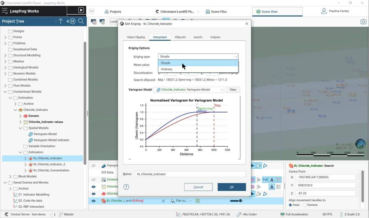
We will be able to model our 3D variogram as an input

[00:01:07.330]
to the estimator with the assistance of Leapfrogs

[00:01:10.290]
highly connected 3D scene.

[00:01:14.410]
It allows for real time visualization

[00:01:16.690]
of your experimental variograms with our 3D scene,

[00:01:20.290]
making the process more intuitive.

[00:01:23.610]
Anytime we change a parameter within

[00:01:26.060]
our experimental variogram or the variogram model,

[00:01:29.300]
we’ll see how our variography change.

[00:01:33.470]
When we right-click on the estimation folder,

[00:01:35.890]
we can select which estimator we want to use.

[00:01:39.690]
For this workflow, we’ll use simple grading.

[00:01:43.320]
We set the parameters for our estimation,

[00:01:45.970]
including the created 3D variography.

[00:01:49.030]
Define the search ellipsoid ranges, the search definition,

[00:01:53.680]
and finally, the required outputs.

[00:01:58.980]
Once the domain, the spatial model,

[00:02:01.140]
and the estimators are set, we must create a block model,

[00:02:04.630]
to code our estimated indicator values.

[00:02:08.270]
Creating a block model is a straightforward workflow

[00:02:12.150]
and a great way of representing contaminants models

[00:02:15.450]
in 3D.

[00:02:17.320]
We can adjust our parameters and select which models

[00:02:20.840]
and estimation will be represented at (inaudible).

[00:02:26.450]
In this case,

[00:02:27.283]
we have evaluated several geological and numerical models,

[00:02:30.920]
as well as different estimators.

[00:02:33.450]
All this information can be reviewed in the scene in a very

[00:02:36.850]
flexible way.

[00:02:39.800]
When indicators are coded into block models,

[00:02:42.550]
we can analyze the probability of each block to be above

[00:02:46.630]
or the final threshold.

[00:02:48.150]
In this case four PPM chloride.

[00:02:52.000]
We can filter the block to this value

[00:02:53.970]
and observe the distribution of the plume.

[00:02:58.460]
Calculations are available in block models to visualize

[00:03:01.720]
new created variables and to report

[00:03:03.840]
mass and average concentration, for example.

[00:03:08.300]
In this case,

[00:03:09.300]
we have created a new category defined by

[00:03:12.310]
the estimated indicator.

[00:03:14.840]
If the indicator value is above 0.6 or 60% probability,

[00:03:20.560]
the blocks will be assigned as a category

[00:03:22.660]
of “High” grow ability.

[00:03:25.010]
If the indicator value ranges from 0.2 to 0.6,

[00:03:29.580]
then it will be classified as medium probability.

[00:03:33.160]
And if the indicator value is below 0.2,

[00:03:36.550]
it will be assigned a ‘Low’ probability.

[00:03:40.440]
As all variables created within the block models,

[00:03:43.010]
we can review this data on a scene.

[00:03:48.100]
Other tools available in block models are statistics,

[00:03:52.630]
interrogate estimator, swath plots, and also reports.

[00:04:01.670]
When creating a report, we must decide,

[00:04:03.930]
what do we want to show.

[00:04:06.500]
In this report, we are categorizing the data

[00:04:09.010]
for geology domain and by probability.

[00:04:13.740]
You can use any data to create indicator modeling.

[00:04:17.070]
Just be clear your objectives

[00:04:18.840]
and select the right tools available.

[00:04:21.730]
If you would like to learn more,

[00:04:23.540]
please contact us at [email protected].

[00:04:27.770]
Thank you.