Es el primer seminario web de una serie de 3 seminarios web sobre la prospección magnética de objetos antropogénicos.

La teoría, la toma de datos y el tratamiento de estos. Estos seminarios web los imparten conjuntamente Seequent y Geometrics. Uno de los objetivos más importantes de los geofísicos es la búsqueda de objetos artificiales en la superficie cercana.

Entre los elementos de interés se encuentran los artefactos sin explotar (UXO) procedentes tanto de las actividades de entrenamiento como de la guerra, las investigaciones arqueológicas y las infraestructuras antiguas como tuberías, cables y tanques de almacenamiento subterráneos donde los mapas y dibujos disponibles no están presentes o son inadecuados. Los métodos magnéticos han sido uno de los principales métodos para detectar estos objetos.

En este seminario web se analizan las implicaciones prácticas de la teoría magnética para la realización de prospecciones, incluidas las repercusiones de lo siguiente:

Tamaño, forma y orientación de objetos ferrosos
Remanencia magnética
Mediciones del gradiente en comparación con el campo total

Duración

42 min

Vea más videos bajo demanda.

Videos

Conozca más sobre Oasis montaj

Más información

Transcripción del video

[00:00:00.730] 
<encoded_tag_open />v -<encoded_tag_closed />Hello, and thank you for joining us today.<encoded_tag_open />/v<encoded_tag_closed /><!– wpml:html_fragment –>
[00:00:03.740] 
My name is Gretchen Schmauder and I am a geoscientist.
[00:00:07.200] 
And the Director of Marketing for Geometrics.
[00:00:10.220] 
Today we also have Becky Bodger, who’s a geoscientist
[00:00:13.640] 
for Seequent. 
<encoded_tag_open />v -<encoded_tag_closed />Hello.<encoded_tag_open />/v<encoded_tag_closed />
[00:00:15.260] 
<encoded_tag_open />v -<encoded_tag_closed />and Bart Hoekstra, who’s a geophysicist<encoded_tag_open />/v<encoded_tag_closed />
[00:00:18.130] 
and the Vice President of sales for Geometrics.
[00:00:22.260] 
<encoded_tag_open />v -<encoded_tag_closed />Hello and thank you all for joining us today.<encoded_tag_open />/v<encoded_tag_closed />
[00:00:27.240] 
<encoded_tag_open />v -<encoded_tag_closed />Stefan Burns also contributed to today’s webinar.<encoded_tag_open />/v<encoded_tag_closed />
[00:00:31.400] 
He created the video you will be seeing here
[00:00:33.610] 
in a few moments.
[00:00:37.410] 
This is the first in a series of three webinars
[00:00:40.500] 
about magnetic geophysics.
[00:00:43.110] 
Today’s webinar covers magnetic theory.
[00:00:47.610] 
Future webinars are going to talk about
[00:00:51.054] 
magnetic data collection,
[00:00:53.350] 
and then the third will be magnetic data processing.
[00:01:00.090] 
We really want today’s webinar to be both informative
[00:01:04.030] 
and interactive.
[00:01:07.020] 
So to keep people engaged, we have included
[00:01:11.010] 
a series of questions that will pop up on the screen
[00:01:14.990] 
as we progress.
[00:01:17.150] 
We’d ask that you answer these questions
[00:01:19.900] 
either using the poll that will pop up on your screen
[00:01:23.800] 
or in the chat window as part of this webinar.
[00:01:28.800] 
Towards the end of today’s session
[00:01:31.580] 
we will talk about some of the answers
[00:01:34.540] 
and hopefully answer any questions you may have.
[00:01:40.910] 
Today we are focusing primarily on anthropogenic objects
[00:01:45.500] 
or those objects related to human beings
[00:01:48.280] 
and their interaction with the earth.
[00:01:51.600] 
The biggest driver for this
[00:01:53.200] 
is a search for unexploded ordinance
[00:01:55.690] 
also known as UXO in both the North Sea
[00:01:58.940] 
and in Southeast Asia.
[00:02:01.540] 
For example, the U.S. dropped over 2 million tons
[00:02:05.760] 
of explosives in Laos in the 1960s and 70s.
[00:02:10.400] 
The image you see on the left shows a field
[00:02:12.890] 
with bomb craters still present after nearly 50 years.
[00:02:18.070] 
On the right-hand side, you can see an unexploded bomb
[00:02:20.660] 
that is still posing significant risk to human inhabitants.
[00:02:26.000] 
In the North Sea world war II era bombs
[00:02:28.630] 
are still littering the sea floor.
[00:02:33.470] 
With the recent increase in wind farm development,
[00:02:37.470] 
efficient exploration for UXO is very important.
[00:02:42.220] 
Other areas driving the need for magnetometers
[00:02:44.830] 
include pipeline tracking and environmental concerns
[00:02:48.200] 
such as leaking underground storage tanks.
[00:02:51.300] 
You can see one of these here in the far left image.
[00:02:55.720] 
In the middle image, you can see an abandoned wellhead.
[00:03:00.740] 
These are frequently cut off below the ground surface,
[00:03:04.470] 
so they are not visible to the eye.
[00:03:10.290] 
Finally, in the right hand image,
[00:03:12.380] 
you can see a magnet, where a magnetometer was used
[00:03:15.450] 
to help characterize an archeological site.
[00:03:20.120] 
So here is our first question.
[00:03:23.220] 
Please write your answers in the chat window.
[00:03:27.170] 
What other anthropogenic objects or hazards can you think of
[00:03:31.670] 
that we can use magnetic surveys to identify?
[00:03:51.160] 
Our presentation begins with a brief explanation
[00:03:54.030] 
of the earth’s magnetic field.
[00:03:56.150] 
After this Bart and Becky will go into a deeper discussion
[00:04:00.010] 
of magnetics and magnetic anomalies.
[00:04:03.810] 
We are here to answer your questions.
[00:04:06.050] 
So please feel free to use the chat feature to contact us
[00:04:09.420] 
at any time during today’s presentation.
[00:04:12.520] 
You can also email us.
[00:04:14.677] 
So let’s get started.
[00:04:18.030] 
<encoded_tag_open />v Stefan<encoded_tag_closed />Electromagnetism is one<encoded_tag_open />/v<encoded_tag_closed />
[00:04:19.390] 
of four fundamental forces that govern our universe.
[00:04:22.780] 
Like two sides of the same coin
[00:04:24.640] 
electrical and magnetic fields can not exist
[00:04:27.060] 
without the other.
[00:04:28.690] 
Electromagnetic field is created when positive
[00:04:31.160] 
and negative particles interact
[00:04:32.980] 
like the nucleus and electrons of an atom.
[00:04:35.350] 
Magnetic fields hold electrons to their atoms
[00:04:38.050] 
resulting in molecular bonds,
[00:04:39.710] 
that hold compounds together and govern chemical reactions.
[00:04:43.330] 
At a macroscopic scale, some planets like earth
[00:04:46.260] 
and the gas giants of our solar system
[00:04:48.410] 
maintain massive magnetic fields of their own.
[00:04:51.590] 
It’s earth’s magnetic field that protects life
[00:04:54.150] 
from dangerous high energy solar wind emitted by the sun.
[00:04:57.990] 
Humans use magnetometry the study of magnetic fields
[00:05:01.640] 
to understand geology and define anthropogenic objects
[00:05:04.680] 
humans have left behind.
[00:05:06.910] 
Hello, my name is Stefan Burns
[00:05:08.730] 
and welcome to the magnetic surveying
[00:05:10.740] 
for detection of anthropogenic objects.
[00:05:15.210] 
If you’ve ever played with a magnet,
[00:05:16.730] 
you have experienced firsthand
[00:05:18.190] 
the unique physics of magnetic fields.
[00:05:20.930] 
Magnets have opposing north and south poles.
[00:05:23.740] 
As the saying goes, opposites attract.
[00:05:26.080] 
And in this case, the north and south poles of a magnet
[00:05:28.780] 
are attracted to each other.
[00:05:30.710] 
When to north or to south poles are placed near each other,
[00:05:34.000] 
repulsive force exists.
[00:05:35.800] 
The poles repel each other at the atomic level.
[00:05:38.980] 
If you could see magnetic fields,
[00:05:40.960] 
you would observe that magnets are surrounded in space
[00:05:43.550] 
by force fields originating at the positive
[00:05:46.410] 
south magnetic pole
[00:05:48.100] 
and ending at the negative north magnetic pole.
[00:05:51.530] 
If you could see an even greater detail,
[00:05:53.860] 
you would find that this field is created
[00:05:55.640] 
by the movement of electrons.
[00:05:57.890] 
Electrons moving from an area of negative charge
[00:06:00.470] 
to one of positive charge to find as electrical current
[00:06:04.160] 
is what gives magnets our ability to attract or repel.
[00:06:07.750] 
When an electric current is created
[00:06:09.470] 
and electrons are in flow a magnetic field is created.
[00:06:12.780] 
And this is the case because electricity and magnetism
[00:06:15.550] 
are linked at the quantum level.
[00:06:18.150] 
Modern magnetometers can sample the magnetic field
[00:06:20.700] 
hundreds or thousands of times per second.
[00:06:23.520] 
Before this, we were still aware of magnetic fields,
[00:06:26.410] 
thanks to simpler technologies, such as the compass.
[00:06:29.470] 
When suspended in water, the magnetised pin of a compass
[00:06:32.650] 
lines up with the magnetic field lines of our planet.
[00:06:35.490] 
Each end pointing to the earth
[00:06:36.930] 
oppositely charged magnetic pole.
[00:06:39.500] 
The earliest recorded use of a compass
[00:06:41.370] 
is dated to the second century BC
[00:06:43.830] 
when people use naturally occurring lodestone,
[00:06:46.450] 
otherwise known as magnetite to locate north.
[00:06:49.560] 
And in the 11th century,
[00:06:50.830] 
Chinese texts describe the needs for navigation
[00:06:53.490] 
amongst the ever-changing conditions at sea.
[00:06:56.650] 
The north arrow of a compass points to what we refer to
[00:06:59.640] 
as Earth’s magnetic north pole.
[00:07:01.620] 
However, you will recall that opposites attract.
[00:07:04.370] 
So what is really going on
[00:07:05.750] 
when a compass needle points north?
[00:07:07.980] 
It turns out that if you represented
[00:07:09.750] 
the earth’s magnetic field using a bar magnet,
[00:07:12.540] 
the bar magnet south pole
[00:07:14.170] 
would lay in the Northern hemisphere.
[00:07:16.750] 
A compass pointing towards the earth magnetic south pole
[00:07:19.790] 
ends up pointing towards geographic north
[00:07:22.210] 
since the geographic north pole and magnetic south pole
[00:07:25.260] 
lie in close proximity to each other.
[00:07:28.280] 
Across geologic time, the earth’s magnetic field
[00:07:30.870] 
has regularly gone through magnetic pole reversals.
[00:07:33.750] 
In the case of a pole reversal today,
[00:07:36.130] 
the poles were switched places
[00:07:37.780] 
and a compass’s north arrow
[00:07:39.360] 
would still point towards the magnetic south pole
[00:07:41.870] 
now located in the Southern hemisphere.
[00:07:44.530] 
And the geographic north pole
[00:07:45.830] 
would now be home to the magnetic north pole.
[00:07:49.410] 
On a human timescale, the earth’s magnetic field
[00:07:52.090] 
wobbles and shifts on a yearly basis
[00:07:54.630] 
and magnetic south is currently moving away from Canada,
[00:07:57.950] 
approximately 55 kilometers per year towards Siberia.
[00:08:02.330] 
Scientists first discovered magnetic pole reversals
[00:08:04.900] 
just over 100 years ago.
[00:08:06.630] 
And it wasn’t until the 1950s
[00:08:08.370] 
that extensive summary mapping projects
[00:08:10.550] 
showed how well the basaltic ocean floor
[00:08:12.690] 
records these magnetic reversals.
[00:08:15.120] 
As seafloor spreading centers deep underwater,
[00:08:17.700] 
magma spews out along geologic fissures
[00:08:20.140] 
and cools into a rock known as basalt.
[00:08:22.950] 
Basalt is faintly magnetic
[00:08:24.500] 
due to its mafic iron rich composition.
[00:08:27.150] 
But in a molten state,
[00:08:28.320] 
iron is not yet permanently magnetized.
[00:08:30.560] 
As this magma cools,
[00:08:31.940] 
minerals containing iron forms in a line
[00:08:34.140] 
to the earth’s magnetic field,
[00:08:35.660] 
just like tiny compass needles.
[00:08:37.900] 
This magnetization continues
[00:08:39.730] 
until the basalt passes through the Curie point
[00:08:42.240] 
or the temperature at which iron containing minerals
[00:08:44.660] 
become fully magnetic.
[00:08:46.460] 
At this point, they are magnetically frozen in space,
[00:08:49.600] 
and unless reheated will show the alignment
[00:08:51.780] 
of the earth’s magnetic field at the geologic time
[00:08:54.023] 
that Curie point was passed.
[00:08:56.190] 
Recognizing this phenomenon,
[00:08:57.690] 
geophysicists can analyze the magnetic signature of a rock
[00:09:01.090] 
along with radiometric age to chronicle the age
[00:09:04.050] 
and timing of earth’s magnetic cycles.
[00:09:06.810] 
The record shows that the earth’s magnetic field
[00:09:09.150] 
can flip quite rapidly and then remain stable
[00:09:11.760] 
for hundreds of thousands or millions of years
[00:09:14.290] 
before undergoing another magnetic pole reversal.
[00:09:17.810] 
Many man-made objects contain magnetic material,
[00:09:20.670] 
and ferromagnetism allows us to detect these objects
[00:09:23.670] 
with magnetometers.
[00:09:25.595] 
Ferromagnetism occurs when electrons spin
[00:09:27.730] 
in alignment with each other and iron cobalt and nickel
[00:09:31.240] 
are common ferromagnetic materials.
[00:09:33.760] 
The greater number of aligned spinning electrons
[00:09:36.210] 
a ferromagnetic material has, the strongest magnetic field.
[00:09:40.200] 
Since the advent of the iron age,
[00:09:41.870] 
many objects created by humans contain ferrous materials,
[00:09:44.860] 
and therefore can be detected
[00:09:46.340] 
by measuring the magnetic field near the earth surface.
[00:09:50.150] 
There are two primary methods
[00:09:51.520] 
for measuring the magnetic field
[00:09:53.150] 
that are commonly used for detecting man-made objects.
[00:09:56.410] 
Magnetic sensors that measure the magnitude
[00:09:58.660] 
of the magnetic field are referred to as atomic sensors,
[00:10:01.840] 
more commonly known as cesium,
[00:10:03.770] 
rubidium, proton, or Overhauser sensors.
[00:10:07.600] 
They each utilized slightly different physics
[00:10:09.630] 
to measure the magnetic field vary from each other
[00:10:12.120] 
in their accuracy, sensitivity, and sample rates.
[00:10:16.090] 
The local distortions of the earth’s magnetic field
[00:10:18.490] 
are observed by magnetometers as anomalous signatures,
[00:10:21.310] 
which can be used to precisely locate anthropogenic objects.
[00:10:25.290] 
Modern magnetic instrumentation can detect variations
[00:10:28.480] 
as small as one millionth
[00:10:29.930] 
of the value of the Earth’s magnetic field.
[00:10:32.237] 
And this increased sensitivity allows for the detection
[00:10:35.620] 
of smaller objects at greater depths.
[00:10:38.430] 
In addition to their incredible resolution,
[00:10:40.600] 
modern magnetometers also rapidly sample the magnetic field.
[00:10:44.000] 
And when many sensors are combined into arrays,
[00:10:46.820] 
large areas of both land and sea can be surveyed
[00:10:49.650] 
in great detail.
[00:10:51.140] 
The other primary method for measuring a magnetic field
[00:10:53.780] 
is to measure the change in the magnetic field
[00:10:55.990] 
over a distance in a particular orientation.
[00:10:59.340] 
These are known as gradient sensors
[00:11:01.240] 
with fluxgate magnetometers being the most common type
[00:11:03.980] 
of gradient sensor.
[00:11:05.890] 
In the remainder of this presentation,
[00:11:07.720] 
we will discuss the factors affecting the size
[00:11:09.980] 
and shape of magnetic signatures of ferromagnetic objects.
[00:11:15.160] 
<encoded_tag_open />v Bart<encoded_tag_closed />Hello, my name is Bart. Hoekstra<encoded_tag_open />/v<encoded_tag_closed />
[00:11:17.470] 
I’m vice president of geophysical sales at Geometrics
[00:11:21.440] 
and have had a long history of surveying
[00:11:23.820] 
for detection of metal objects primarily for UXO,
[00:11:27.960] 
but also other infrastructure related objects
[00:11:30.690] 
such as underground storage tanks and pipelines.
[00:11:35.640] 
What I will be talking about is some of the complexities
[00:11:38.510] 
that occur when we try and measure an anomaly
[00:11:42.430] 
or the signature of a man-made object.
[00:11:47.180] 
One of the things about magnetic surveys
[00:11:49.310] 
is that they’re quite easy to do.
[00:11:51.800] 
The sensors aren’t that large,
[00:11:53.840] 
and you can carry them or fly them around,
[00:11:56.456] 
download the data and create a map.
[00:11:59.940] 
But the simplicity of this survey
[00:12:02.160] 
and processing disguises the fact
[00:12:05.030] 
that sometimes what we measure
[00:12:06.790] 
is not as simple as we would like it to be.
[00:12:10.010] 
This can lead to misinterpretation of features
[00:12:12.980] 
and possibly not recognizing the presence of an object.
[00:12:17.330] 
One of these complexities arises from something called
[00:12:21.430] 
remanent magnetization.
[00:12:25.630] 
Stefan briefly discussed this in his intro,
[00:12:28.920] 
but what happens with ferromagnetic materials
[00:12:31.750] 
is that they have mineral grains.
[00:12:34.180] 
And within each one of these mineral grains,
[00:12:36.640] 
you can have a different alignment of the electrons
[00:12:39.300] 
which causes a different alignment
[00:12:41.100] 
of the south and north magnetic poles.
[00:12:44.950] 
When the ferromagnetic object that contains the grains
[00:12:48.160] 
is heated and then cooled below its Curie temperature,
[00:12:52.650] 
the magnetic grains will align
[00:12:54.870] 
with the earth’s magnetic field that occurs
[00:12:57.670] 
at the point in time and space and orientation of the object
[00:13:02.310] 
within the surrounding magnetic field.
[00:13:05.460] 
So the upper image shows the effects
[00:13:10.300] 
or what the remanent magnetization will be
[00:13:12.980] 
above the Curie temperature,
[00:13:14.650] 
but once it’s aligned and cooled below,
[00:13:18.690] 
the Curie temperature,
[00:13:19.640] 
you can see that all the magnetic domains within each grain
[00:13:23.220] 
are aligned with the external magnetic field.
[00:13:29.780] 
But what happens over time
[00:13:31.960] 
is that some of the remanent magnetization
[00:13:34.130] 
in these mineral grains becomes weaker
[00:13:36.460] 
and can go away altogether.
[00:13:39.300] 
And then you have a combination of remanent magnetization
[00:13:42.630] 
in some mineral grains and induced magnetization
[00:13:45.840] 
in other mineral grains.
[00:13:48.400] 
And the induced magnetization will line up
[00:13:50.620] 
with the external magnetic field
[00:13:52.720] 
that is present at the space and time
[00:13:55.130] 
in orientation where the object is now
[00:13:57.370] 
which may be different from the magnetic field where it was
[00:14:02.040] 
when it first cooled below the Curie temperature.
[00:14:06.230] 
And these two fields can be very different from each other
[00:14:09.880] 
in both magnitude and direction.
[00:14:12.675] 
And in some cases, the remanent magnetization,
[00:14:15.840] 
depending on the strength of it,
[00:14:17.930] 
can be up to five times the size
[00:14:20.900] 
of the induced magnetization,
[00:14:23.090] 
or it could be an almost negative negligible factor
[00:14:26.230] 
of the, compared to the induced magnetization.
[00:14:33.650] 
And so the result of this
[00:14:35.720] 
is that we have a vector sum,
[00:14:38.190] 
the field you measure will be a vector sum
[00:14:41.520] 
of the induced magnetization and the remanent magnetization,
[00:14:46.320] 
and often what is referred to as a Koenigsberger ratio
[00:14:51.050] 
is the ratio of the magnetic remanent field
[00:14:55.790] 
versus the induced field.
[00:14:58.630] 
So in the next series of slides,
[00:15:00.870] 
I’m going to be talking about
[00:15:02.840] 
and giving examples of the effects of remanent magnetization
[00:15:08.090] 
on a measured anomaly for a particular object.
[00:15:15.446] 
The particular object we are going to
[00:15:19.500] 
show the results, the model results of
[00:15:22.040] 
is an oblate spheroid.
[00:15:25.090] 
And this is kind of a UXO shaped object.
[00:15:28.750] 
It’s 10 centimeters in diameter, 50 centimeters in length.
[00:15:32.070] 
And it’s located at a depth of three meters
[00:15:35.570] 
below the plane of the model measurements.
[00:15:39.640] 
It’s inclined 60 degrees down
[00:15:42.800] 
and is oriented 60 degrees from north.
[00:15:47.940] 
The background field is approximately 50 nanoteslas,
[00:15:52.600] 
which is a close approximation
[00:15:55.060] 
of the earth’s magnetic field.
[00:15:56.190] 
And it’s at an inclination of 30 degrees positive,
[00:16:00.180] 
which is somewhat different from those that are
[00:16:02.920] 
used to seeing measurements in the Northern hemisphere,
[00:16:06.090] 
but you’ll still recognize the anomalies that are modeled.
[00:16:14.880] 
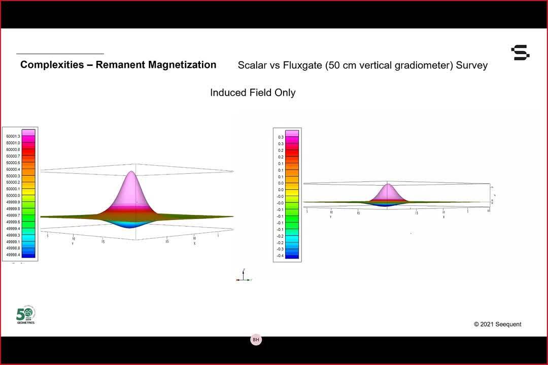
So now we’re going to show the modeled results
[00:16:17.330] 
from this target.
[00:16:18.270] 
And this first slide is,
[00:16:20.120] 
contains just the induced magnetic field.
[00:16:23.820] 
On the left-hand side we have the model data
[00:16:26.780] 
from the object as measured by a total field sensor.
[00:16:31.330] 
And on the right hand side,
[00:16:32.690] 
we have the model data as measured
[00:16:35.770] 
as would be measured from a gradient sensor
[00:16:39.510] 
with 50 centimeter with, on a gradient.
[00:16:45.180] 
This first slide shows just the induced field only.
[00:16:50.150] 
And as you can see, we have a large peak
[00:16:53.110] 
that’s to the Northeast of the
[00:16:58.420] 
target and a smaller trough to the south west.
[00:17:10.050] 
The next animation shows what happens
[00:17:13.450] 
when we have a remanent field that is the same amplitude
[00:17:17.940] 
as the induced magnetic field,
[00:17:20.940] 
and it’s oriented vertically downwards.
[00:17:22.830] 
As you can see,
[00:17:23.740] 
it changes the shape of the anomalies significantly,
[00:17:28.010] 
and we have a much larger trough
[00:17:30.490] 
now that’s still oriented towards the Southwest
[00:17:34.040] 
and it’s decreased the peak.
[00:17:38.520] 
All right, the third animation shows what happens
[00:17:41.880] 
when we have a remanent magnetization
[00:17:45.070] 
still the same amplitude, but now it’s oriented in the,
[00:17:50.120] 
towards the west horizontally.
[00:17:52.400] 
And as you can see it all,
[00:17:54.480] 
again, change the shape of the anomaly
[00:17:56.460] 
and now our smaller trough
[00:17:59.300] 
is oriented towards the Southeast.
[00:18:03.320] 
So this is quite a change from the original induced
[00:18:07.465] 
all the measurement that we have.
[00:18:11.060] 
The final animation in this slide
[00:18:13.500] 
is with the induced or the remanent field
[00:18:18.140] 
oriented towards the west.
[00:18:23.320] 
And as you can see this looks actually
[00:18:25.410] 
kind of similar to what we had with just the induced field,
[00:18:29.190] 
except now that the trough is oriented
[00:18:32.880] 
towards the Northwest.
[00:18:37.080] 
This just shows you some of the complexities
[00:18:39.440] 
that can arise when you have strong remanent magnetization,
[00:18:43.150] 
and it can distinctly change the shape of your anomaly
[00:18:46.360] 
and may cause you to misinterpret what you have.
[00:18:51.760] 
The next set of animations we’re going to model
[00:18:54.350] 
is using the same object
[00:18:56.760] 
and the same induced magnetization field,
[00:18:59.588] 
and use the same set of four parameters
[00:19:03.250] 
for the remanent magnetization.
[00:19:05.440] 
But what we’re doing, what we’ve done now
[00:19:07.910] 
is added noise that you’ll typically see
[00:19:10.470] 
from a total field survey and from a gradient survey
[00:19:14.600] 
so you can see how the remanent magnetization
[00:19:18.020] 
will change possibly the interpretation of the anomaly.
[00:19:22.320] 
The first animation is with the induced magnetic field only,
[00:19:27.710] 
and you can see the object quite well.
[00:19:31.640] 
The next animation has remanent magnetization
[00:19:35.780] 
that is oriented vertically downwards.
[00:19:40.440] 
The third animation has the remanent magnetization
[00:19:44.673] 
that is horizontal, but it’s in the Southern direction.
[00:19:48.933] 
And the final animation has the remanent magnetic field
[00:19:53.171] 
oriented horizontally but pointing to the west.
[00:19:57.840] 
And as you can see from our examples with noise,
[00:20:00.330] 
in some cases, the remanent magnetization
[00:20:03.200] 
can make an anomaly from a very metallic object
[00:20:06.640] 
look quite different than what you’re expecting
[00:20:08.970] 
from just an induced field anomaly.
[00:20:12.660] 
And in many cases that may lead you
[00:20:16.130] 
to not selecting the object as an object of interest
[00:20:21.660] 
or misinterpreting what that object is.
[00:20:26.184] 
We’re now going to discuss
[00:20:27.370] 
some of the different types of measurements
[00:20:29.340] 
that Stefan discussed in the introduction.
[00:20:33.640] 
We’re going to talk about two,
[00:20:35.250] 
basically two kinds of measurements.
[00:20:37.020] 
The first one is what we call a total field sensor,
[00:20:40.680] 
which measures just the magnitude of the field
[00:20:45.270] 
in, at a point in and time.
[00:20:49.010] 
These total field measurements
[00:20:50.470] 
are called total field sensors, scalar magnetometers,
[00:20:54.220] 
or atomic magnetometers.
[00:20:57.290] 
And then we’re also going to look at
[00:20:58.970] 
what are called gradient measurements.
[00:21:01.590] 
And what they look at is the difference
[00:21:03.800] 
in the magnetic field over a distance
[00:21:07.560] 
in a specific orientation.
[00:21:10.490] 
In most cases, gradient measurements are made with
[00:21:14.020] 
in either the vertical or a horizontal plane.
[00:21:18.640] 
With vertical gradient measurements,
[00:21:20.700] 
we measure the difference in the magnetic field
[00:21:23.560] 
from the top and the bottom of your sensor or sensor array.
[00:21:29.160] 
For horizontal gradient measurements,
[00:21:31.510] 
you’re looking at the difference across the width
[00:21:34.450] 
of your sensor or sensors array.
[00:21:38.300] 
Gradient measurements can be made with total field sensors
[00:21:41.930] 
that are separated
[00:21:43.480] 
by a specified distance, or they can be made
[00:21:46.060] 
with what are referred to as fluxgate sensors.
[00:21:51.200] 
On the left-hand side, we have a measurement
[00:21:53.280] 
that’s made by a fluxgate magnetometer
[00:21:55.720] 
in this case, the FM18.
[00:21:58.740] 
And this was done over the NSGG test site located in the UK.
[00:22:05.500] 
You can see various features on this map.
[00:22:08.280] 
And in particular,
[00:22:09.460] 
you can see clearly distinct anomalies
[00:22:12.370] 
to the, in the central Northern part of the map
[00:22:16.110] 
that were buried objects as tests for anomaly detection.
[00:22:21.720] 
And that’s shown on the left-hand side.
[00:22:25.260] 
On the right hand side,
[00:22:27.010] 
we have measurements that were made using
[00:22:30.140] 
two total field sensors separated by about a meter.
[00:22:34.860] 
And you can see the two maps are quite similar.
[00:22:37.660] 
There’s some differences.
[00:22:39.730] 
But in general, you can see the anomalies quite well.
[00:22:43.640] 
And it’s fairly easy to pick out our objects of interest.
[00:22:49.800] 
In the next slide, what we’re showing
[00:22:51.730] 
is the total field measurement made by a single sensor
[00:22:56.020] 
from the array of G858.
[00:22:58.530] 
And you can see this map looks different
[00:23:01.320] 
than the other sensors or other maps that we were showing.
[00:23:05.900] 
You can clearly see some of the large anomalies
[00:23:09.540] 
in the Northern half of this map,
[00:23:13.200] 
which were the buried objects.
[00:23:15.200] 
And you can see some other anomalies outside that region,
[00:23:18.900] 
but they tend to be a little bit more subtler.
[00:23:21.620] 
And that’s likely due to the fact
[00:23:23.540] 
that they were smaller objects nearer to the center
[00:23:27.880] 
or near to the surface.
[00:23:29.870] 
And in general these are not picked up as easily as
[00:23:35.620] 
the gradient measurements too.
[00:23:37.620] 
But, this map I would say tends to be a little bit
[00:23:42.130] 
less noisy.
[00:23:44.420] 
Where there are no objects
[00:23:46.070] 
you don’t see much magnetic field variation.
[00:23:49.380] 
The other thing you’ll note about this odd map is that
[00:23:53.010] 
there is a gradient, a long wavelength gradient
[00:23:59.748] 
in the data with the magnetic field decreasing
[00:24:02.200] 
to the south of this area
[00:24:05.260] 
that you did not see in a gradient field measurement.
[00:24:08.380] 
And this is because when you take two sensors
[00:24:12.380] 
or you’re just measuring the difference between two points,
[00:24:17.482] 
they will see the same long wavelength gradient
[00:24:21.090] 
and when you subtract out the field from the top and bottom,
[00:24:26.500] 
then there is no long-term wavelength difference
[00:24:31.020] 
in the measurement.
[00:24:32.750] 
So I just wanted to highlight that and I’ll just go in,
[00:24:37.300] 
in the next slide.
[00:24:39.100] 
So in this slide, I’ll discuss some of the reasons why
[00:24:42.760] 
there is a difference between measuring the magnetic field
[00:24:46.480] 
with a total field sensor or a scaler sensor
[00:24:49.920] 
versus a gradient sensor.
[00:24:54.570] 
The total field signal decreases in amplitude
[00:24:59.830] 
by a factor of one over R to the third with distance.
[00:25:05.890] 
The gradient signal decreases
[00:25:08.210] 
by a factor of one over R to the fourth.
[00:25:11.210] 
On the chart, on the right hand side,
[00:25:14.580] 
the decrease in amplitude is,
[00:25:18.440] 
with distance is represented by this blue curve
[00:25:22.780] 
for a total field measurement
[00:25:24.520] 
and a decrease in amplitude of the measurement
[00:25:27.580] 
for a gradient signal is shown in the red curve.
[00:25:33.790] 
And this distance and amplitude are normalized
[00:25:37.140] 
by the amplitude of the anomaly
[00:25:39.900] 
and also the length of the dipole.
[00:25:43.690] 
But as you can see at a factor,
[00:25:46.170] 
a distance of eight compared to the length of the dipole,
[00:25:51.160] 
the total field measurement in blue
[00:25:54.010] 
is actually an order of magnitude almost greater
[00:25:58.450] 
than the amplitude of the gradient measurement.
[00:26:05.750] 
And so this has a pretty big impact on your ability
[00:26:10.760] 
to detect objects at a greater range from your sensor.
[00:26:16.240] 
So in general, a total field measurement
[00:26:19.130] 
is more effective at detecting objects at greater distances.
[00:26:24.710] 
But, there are some advantages
[00:26:27.610] 
to doing gradient measurements.
[00:26:29.560] 
They tend to filter out low frequency trends
[00:26:31.910] 
as you saw in your previous map.
[00:26:34.530] 
The anomaly that you see from a gradient measurement
[00:26:37.810] 
is sometimes a little bit better defined.
[00:26:40.980] 
It’s sharper and narrower in width
[00:26:43.570] 
which makes it easier to determine the location
[00:26:47.560] 
of an object.
[00:26:50.700] 
And if you’re interested in shallow objects,
[00:26:54.860] 
it can also enhance the location and detection ability
[00:26:58.220] 
of those shallow objects.
[00:27:00.750] 
One other factor to consider
[00:27:02.280] 
when you look at gradient measurements
[00:27:04.150] 
is that they tend to be noisier.
[00:27:07.537] 
That’s because we’re actually taking the derivative
[00:27:10.160] 
of the magnetic field in that particular orientation,
[00:27:14.390] 
either vertically or horizontally
[00:27:16.670] 
and in all cases derivative measurements
[00:27:20.020] 
tend to act as a high pass filter.
[00:27:22.510] 
And noise in most magnetic surveys is,
[00:27:26.950] 
increases with frequency
[00:27:29.411] 
and so you will tend to increase noise
[00:27:34.160] 
in your measured signals.
[00:27:36.930] 
So, as a question I’d like to ask people,
[00:27:40.230] 
what kind of measurement the magnetic field measurements
[00:27:43.620] 
they have made in the past or plan to in the future.
[00:27:48.050] 
Do you use a total field sensor or atomic sensor,
[00:27:53.535] 
a gradient sensor such as a fluxgate
[00:27:55.760] 
or use a gradient array of total field sensors?
[00:28:00.420] 
Have you done both kinds of surveys
[00:28:02.280] 
or are you brand new to magnetic surveying
[00:28:05.170] 
and haven’t done anything?
[00:28:06.790] 
So please answer the poll in the chat window
[00:28:10.150] 
and we can discuss the results later on.
[00:28:32.960] 
Well, that concludes my section of the talk.
[00:28:35.560] 
And now I’m going to hand off the presentation
[00:28:37.880] 
to Becky Bodger from Seequent.
[00:28:40.870] 
I will be back to discuss the conclusions of this webinar,
[00:28:45.040] 
and also to answer any questions that you may have.
[00:28:49.837] 
<encoded_tag_open />v Becky<encoded_tag_closed />Thanks, Bart.<encoded_tag_open />/v<encoded_tag_closed />
[00:28:51.110] 
As mentioned, my name is Becky Bodger
[00:28:52.730] 
and I’m a geoscientist at Seequent.
[00:28:55.960] 
In this next section
[00:28:56.793] 
I’m going to show you a series of examples
[00:28:58.690] 
that were created using the forward modeling capabilities
[00:29:01.660] 
available in Oasis montaj with the UXO extension.
[00:29:05.330] 
The grid on the left is the background that I used
[00:29:07.660] 
for the forward modeling.
[00:29:08.910] 
It’s from an actual UXO survey in the North Sea,
[00:29:12.220] 
and is representative of the type and level of noise
[00:29:15.050] 
you would get on a real survey.
[00:29:17.080] 
In most of the examples,
[00:29:18.370] 
I’m using a 155 millimeter projectile
[00:29:21.700] 
unless otherwise stated.
[00:29:23.480] 
And there’s an image on the right
[00:29:25.840] 
that shows you what that looks like.
[00:29:31.880] 
So whenever you are working with any potential field data,
[00:29:34.880] 
for example, gravity or magnetics,
[00:29:37.000] 
we need to remember that mathematically
[00:29:38.840] 
magnetic anomalies are non-unique.
[00:29:40.940] 
Multiple theoretical solutions are possible.
[00:29:43.890] 
This is true whether we’re talking about geological features
[00:29:47.430] 
or anthropogenic objects.
[00:29:50.480] 
I found this image in a paper online
[00:29:52.400] 
that talks about the ambiguity in potential field modeling.
[00:29:55.800] 
And I like it because it demonstrates
[00:29:57.390] 
that the same Mickey mouse shaped deposit
[00:29:59.610] 
can have three different geophysical signatures.
[00:30:02.390] 
Why do we continue to use magnetics though,
[00:30:04.450] 
or any potential field data?
[00:30:06.190] 
Because there are ways to minimize this issue.
[00:30:10.760] 
So using a priori information in most cases
[00:30:13.660] 
especially when we were talking about anthropogenic objects,
[00:30:16.480] 
there’s history somewhere.
[00:30:18.720] 
If it’s UXO, we can research
[00:30:20.610] 
which munitions were dropped by either side
[00:30:23.130] 
during the various wars or conflicts.
[00:30:25.330] 
For archeology, hopefully you know some of the history
[00:30:28.100] 
of the area and what you are looking for,
[00:30:30.060] 
whether it’s an old burial site or building foundations.
[00:30:33.440] 
And for geotechnical investigations,
[00:30:35.660] 
there are often existing infrastructure maps
[00:30:37.980] 
showing the locations of buried cables and pipelines.
[00:30:41.290] 
This information is not always available,
[00:30:43.470] 
or it can be difficult to unearth,
[00:30:45.320] 
but it’s worth checking what’s available
[00:30:47.190] 
to aiding your processing and interpretation of the data
[00:30:50.050] 
before you start.
[00:30:53.780] 
Cross-referencing multiple types of geophysical data.
[00:30:57.450] 
So in the case of offshore geophysical surveys,
[00:31:00.500] 
mag is only part of the story.
[00:31:02.410] 
Oftentimes surveyors will simultaneously
[00:31:05.400] 
be collecting multi-team data, side scan, sonar,
[00:31:08.650] 
seismic, sub-bottom profile data, or even seabed images.
[00:31:13.110] 
Using the results of all of this data
[00:31:15.260] 
will really help with processing
[00:31:17.470] 
and the interpretation of your results.
[00:31:20.240] 
And in archeological studies, for example,
[00:31:22.760] 
you might have gravity and resistivity as well.
[00:31:28.560] 
Finally, use your common sense and be smart.
[00:31:31.770] 
You’re going to use common sense, your education,
[00:31:34.320] 
your past experience, all of that,
[00:31:36.320] 
to apply logic and find the best interpretation.
[00:31:40.760] 
Here, I attempt to demonstrate
[00:31:42.390] 
the non uniqueness of this mag anomaly.
[00:31:44.710] 
While they are not identical,
[00:31:46.620] 
I hope that we can agree that they are similar enough
[00:31:48.840] 
to demonstrate the point.
[00:31:50.780] 
So on the left we have two UXOs.
[00:31:52.890] 
One is an 81 millimeter projectile
[00:31:54.970] 
at 2.5 meters below the sensor.
[00:31:57.400] 
And one is a two and three quarter inch rocket
[00:31:59.490] 
at two meters below the sensor.
[00:32:01.440] 
On the right, we have a single UXO,
[00:32:04.200] 
which is the 155 millimeter that we’ve been looking at
[00:32:07.560] 
at 3.5 meters.
[00:32:09.590] 
And you can see that on the left-hand side,
[00:32:13.929] 
you know, the inflection point
[00:32:15.550] 
between the dipole’s a little bit slanted.
[00:32:17.610] 
It’s a little smaller than the one on the right.
[00:32:20.230] 
If we look at the profile below the grid,
[00:32:22.320] 
we can see that in profile they’re even harder
[00:32:24.890] 
to distinguish the differences.
[00:32:26.780] 
They both have similar positive and negative peaks.
[00:32:30.730] 
And again, the real only difference that we see here
[00:32:33.250] 
is the width of the actual dipole.
[00:32:38.360] 
This example also demonstrates the importance
[00:32:40.710] 
of griding your data and not only interpreting the results
[00:32:44.650] 
in, along the profile.
[00:32:46.490] 
It’s important to visualize it in 2D space
[00:32:48.770] 
to really see the full picture.
[00:32:51.120] 
So here’s another question for you guys.
[00:32:53.521] 
Which inclination of an object
[00:32:55.990] 
produces the strongest amplitude
[00:32:58.020] 
whether it’s peak to peak of the dipole
[00:33:00.090] 
or a single peak amplitude?
[00:33:02.290] 
Do you think it’s A, vertical, B horizontal,
[00:33:04.990] 
or C inclined at 45 degrees?
[00:33:09.130] 
So I’ll give you a few seconds
[00:33:10.150] 
just to putting your answers and then we’ll carry on.
[00:33:26.060] 
In this example, I’m going to show you the response
[00:33:28.220] 
of the object at different inclinations.
[00:33:32.570] 
So on the right,
[00:33:34.210] 
the image is just to represent the orientation
[00:33:36.920] 
we didn’t actually model the UXO that you’re seeing.
[00:33:40.890] 
So you can see that when it’s horizontal,
[00:33:42.640] 
it’s a nice perfect dipole.
[00:33:45.350] 
When you add inclination,
[00:33:46.820] 
so on the example that we modeled here
[00:33:48.780] 
was inclined at 45 degrees.
[00:33:50.800] 
You can see that the negative trough
[00:33:52.910] 
becomes a lot less negative.
[00:33:55.630] 
And when it’s perfectly vertical,
[00:33:58.630] 
you can see that the negative disappears altogether
[00:34:01.850] 
and you’re left with a monopole.
[00:34:04.770] 
And again, just remember,
[00:34:05.890] 
we’re not modeling the size of the UXO in the image,
[00:34:08.550] 
it’s just there to show you that it’s vertical is possible
[00:34:11.780] 
especially in the marine environment.
[00:34:14.560] 
So what’s the answer to the question that I asked?
[00:34:17.500] 
Here we have the three responses along a profile
[00:34:20.140] 
through the center of the dipole.
[00:34:22.370] 
The first is the horizontal,
[00:34:24.240] 
and we can see that the peak to peak amplitude
[00:34:27.750] 
is 5.4 nanoteslas.
[00:34:31.410] 
The second one in the middle here,
[00:34:32.730] 
is the object inclined at 45 degrees
[00:34:35.830] 
and it has a peak to peak value of six nanoteslas.
[00:34:39.600] 
And the vertical object has a positive monopole
[00:34:46.140] 
total peak value of 6.4 nanoteslas.
[00:34:50.600] 
So the answer to that last question was C for vertical.
[00:34:57.420] 
Next, we’re going to look at how the response changes
[00:35:00.170] 
as the object changes direction or destination.
[00:35:03.560] 
The top row is the horizontal 155 millimeter projectile
[00:35:07.721] 
at four meters below the sensor.
[00:35:10.640] 
And the bottom row is the inclined object at 45 degrees.
[00:35:15.600] 
Note how the negative part of the dipole
[00:35:17.490] 
decreases more rapidly as we rotate the inclined object.
[00:35:22.430] 
The first row is the near vertical object
[00:35:25.090] 
inclined at 85 degrees.
[00:35:26.930] 
And the second row is the same object
[00:35:29.960] 
inclined at negative 60 degrees
[00:35:33.580] 
which implies the opposite polarity.
[00:35:36.240] 
So, instead of the north pole up in the air,
[00:35:40.140] 
in this example, the south pole is up in the air.
[00:35:45.938] 
An interesting effect in the negative 60 degree example
[00:35:50.040] 
is also the halo that we see around the more obvious dipole.
[00:35:54.120] 
This is important
[00:35:55.130] 
when trying to model the depth of the object,
[00:35:57.783] 
whether you are using Euler deconvolution
[00:36:00.770] 
or an inversion style modeling method.
[00:36:03.540] 
Most methods require you to define the modeling window
[00:36:06.810] 
in order to select which data to invert.
[00:36:09.390] 
Since all of these examples use the exact same background
[00:36:12.600] 
which you can see in the top right-hand corner here,
[00:36:15.270] 
any differences in color that we see
[00:36:17.840] 
is part of the signal from the object.
[00:36:20.220] 
So for accurate modeling, we would ideally want to include
[00:36:23.060] 
as much of that signal as possible,
[00:36:25.130] 
which means it would require a much larger modeling window.
[00:36:30.400] 
Let’s also consider the effect of depth below the sensor
[00:36:34.090] 
on the inclined examples.
[00:36:35.840] 
So in the top row, we have the eastward facing
[00:36:38.560] 
155 millimeter projectile inclined at negative 60.
[00:36:42.750] 
And on the bottom, we have the same size projectile,
[00:36:45.020] 
but inclined at 45 degrees.
[00:36:47.170] 
And we can see the different response we get
[00:36:49.580] 
at 1.5 meters below the sensor, 2.5, 3.5, 4.5.
[00:36:55.780] 
And we can see that, we can actually see
[00:36:58.200] 
that none of these examples really produce
[00:37:00.010] 
that perfect looking dipole.
[00:37:01.920] 
And in fact, as the distance between the sensor
[00:37:04.400] 
and the object increases depending on the example,
[00:37:07.680] 
the positive in the top example
[00:37:09.420] 
and the negative in the bottom example,
[00:37:11.450] 
disappears almost entirely
[00:37:13.100] 
and leaves us with another parent monopole.
[00:37:17.500] 
So the last example or complexity
[00:37:19.710] 
I wanted to talk about today
[00:37:21.450] 
is simply the difficulty that arises
[00:37:23.370] 
when you have multiple objects stacked on top
[00:37:26.260] 
or close to one another.
[00:37:27.660] 
And this is a common phenomenon in test ranges
[00:37:30.770] 
or munition dumpsites.
[00:37:32.460] 
So on the left, I’ve modeled two UXOs.
[00:37:35.060] 
One is a 105 millimeter projectile
[00:37:37.540] 
at 3.5 meters below the sensor.
[00:37:40.650] 
Southward facing.
[00:37:42.210] 
And one meter away is a second UXO,
[00:37:45.133] 
a 60 millimeter projectile at two meters below the sensor
[00:37:48.180] 
and westward facing.
[00:37:50.360] 
It creates what I think would be called a complex dipole.
[00:37:54.310] 
On the right-hand side, is another example.
[00:37:56.510] 
A 155 millimeter at four meters
[00:37:59.080] 
and a 105 millimeters at two meter depth below sensor.
[00:38:03.170] 
Both roughly southward facing.
[00:38:05.200] 
With careful analysis, the example on the right
[00:38:08.100] 
could probably be accurately classified
[00:38:10.300] 
as two separate targets,
[00:38:12.340] 
but the example on the left would be a lot,
[00:38:15.300] 
would be much more difficult to separate.
[00:38:19.000] 
And I just wanted to give you a few,
[00:38:20.420] 
a couple of examples where we see this in real life
[00:38:23.330] 
and which caused a lot of problems.
[00:38:25.270] 
So in this example, this is a map
[00:38:27.450] 
of Lac Saint-Pierre in Canada.
[00:38:30.730] 
And I just wanted to show you the complexity
[00:38:32.470] 
and the problem that they’re dealing with here.
[00:38:34.950] 
And as an example, one of these large blue circles is,
[00:38:39.950] 
there are over 200 UXOs in that tiny little space.
[00:38:44.720] 
Another example in Europe is,
[00:38:47.820] 
this is the port in marked munition dump
[00:38:49.850] 
off the coast of Zeebrugge Harbor.
[00:38:52.190] 
This site contains a mix of world war I
[00:38:54.520] 
and world war II munitions,
[00:38:55.940] 
as well as a number of shipwrecks.
[00:38:58.050] 
This is a preliminary magnetic anomaly map.
[00:39:00.790] 
But now the real work begin is trying to separate the signal
[00:39:04.130] 
and finding the best method for cleaning up
[00:39:06.290] 
and monitoring the site.
[00:39:07.890] 
Because in these examples,
[00:39:09.680] 
mag alone will not get the job done.
[00:39:11.550] 
And you’ll, they’ll definitely need to use mag
[00:39:13.960] 
along with other geophysical methods to solve this problem.
[00:39:22.090] 
<encoded_tag_open />v Bart<encoded_tag_closed />In this section I talked about,<encoded_tag_open />/v<encoded_tag_closed />
[00:39:23.420] 
we talked about two factors that can influence
[00:39:26.063] 
the magnetic data that you measure.
[00:39:28.730] 
One is the remanent magnetization
[00:39:30.580] 
that can occur in ferromagnetic objects.
[00:39:33.320] 
And what we saw is that the presence
[00:39:35.750] 
orientation and strength of remanent magnetization
[00:39:39.838] 
can have a very strong impact
[00:39:41.970] 
on the anomaly amplitude in shape,
[00:39:44.800] 
and that it can be quite common in ferrous materials.
[00:39:49.200] 
And that’s sort of highlighted in these two images
[00:39:52.610] 
on the left-hand side of this slide.
[00:39:55.440] 
The other thing I discussed is the difference
[00:39:57.900] 
between a total field and gradient measurement
[00:40:01.130] 
of the magnetic field
[00:40:02.970] 
and how they differ and their ability to locate
[00:40:06.960] 
targets that are deeper
[00:40:08.210] 
or farther away from the sensor versus shallower,
[00:40:11.600] 
their noise levels and the impact
[00:40:14.950] 
of low frequency wavelength, spatial wavelengths signals
[00:40:19.340] 
on the data sets that you acquire.
[00:40:22.800] 
<encoded_tag_open />v Becky<encoded_tag_closed />So if there’s one key point<encoded_tag_open />/v<encoded_tag_closed />
[00:40:25.098] 
I’d like you to take away from my examples,
[00:40:26.660] 
it’s the presence of these monopoles.
[00:40:29.240] 
We always assume that the UXO
[00:40:31.300] 
is going to give us a nice clean dipole,
[00:40:33.330] 
and as we could see, that’s not the case.
[00:40:36.090] 
So, I mean, it was just a few minutes ago,
[00:40:38.130] 
but can you even remember all these examples
[00:40:40.660] 
that I showed you?
[00:40:41.810] 
So the first one, it was the
[00:40:43.680] 
155 inclined object at four meter depth.
[00:40:48.320] 
The next one was the 45 degree at 4.5 meter depth.
[00:40:54.930] 
This one was the 155 inclined at 85 degrees.
[00:41:01.710] 
So that’s almost vertical in the middle.
[00:41:03.720] 
And then this one was the negative 60 at four meters.
[00:41:07.630] 
So quite at a, quite a depth.
[00:41:10.220] 
And then that final one
[00:41:13.230] 
was the same negative 60 at 4.5 meters.
[00:41:18.600] 
So I think that was a really interesting
[00:41:21.155] 
observation from those examples.
[00:41:26.070] 
<encoded_tag_open />v Gretchen<encoded_tag_closed />Thank you again for joining us today.<encoded_tag_open />/v<encoded_tag_closed />
[00:41:28.710] 
If you have questions after this presentation,
[00:41:31.044] 
please feel free to email us
[00:41:32.930] 
at the address listed on the side.
[00:41:35.530] 
Don’t forget we will be having future webinars
[00:41:37.950] 
on magnetic data collection and magnetic data processing
[00:41:41.820] 
later on this year.
[00:41:43.660] 
We have not determined the dates for this yet,
[00:41:46.062] 
but we are tentatively scheduling them
[00:41:48.350] 
for November and December.
[00:41:51.150] 
We will be adding this recording
[00:41:52.760] 
to our Geometrics YouTube channel,
[00:41:54.700] 
and it will also be available on both
[00:41:56.800] 
the Seequent and Geometrics websites.
[00:42:00.370] 
Thank you again for your time
[00:42:01.660] 
and we hope our presentation was useful and informative.
<wpml_invalid_tag original=»PHA+» />[00:42:05.170] 
We look forward to hearing from you.

Prospección magnética de objetos antropogénicos: La teoría

Es el primer seminario web de una serie de 3 seminarios web sobre la prospección magnética de objetos antropogénicos.

Vea más videos bajo demanda.

Conozca más sobre Oasis montaj

Transcripción del video

Related