Это первый вебинар в серии из 3-х вебинаров по магниторазведке антропогенных объектов.

Теория, сбор данных и обработка данных. Вебинары проводятся совместно Seequent и Geometrics. Поиск искусственных объектов вблизи поверхности всегда был важной задачей геофизиков.

Объекты, представляющие интерес, включают неразорвавшиеся боеприпасы (НРБ), оставшиеся после учений и боевых действий, археологические предметы и старую инфраструктуру, такую как трубопроводы, кабели и подземные резервуары-хранилища в случаях, когда карты и чертежи отсутствуют или расходятся с реальным положением дел. Магнитная разведка всегда была одним из основных методов обнаружения этих объектов.

Этот вебинар посвящен практическим последствиям магнитной теории для проведения съемок, включая влияние следующих факторов:

Размер, форма и ориентация железных предметов
Остаточная намагниченность
Градиентометрия и измерение общей напряженности поля

Продолжительность

42 минуты

Смотреть больше видео по запросу

Видео

Узнайте больше об Oasis montaj

Узнать больше

Расшифровка видеозаписи

[00:00:00.730] 
<encoded_tag_open />v -<encoded_tag_closed />Hello, and thank you for joining us today.<encoded_tag_open />/v<encoded_tag_closed /><!— wpml:html_fragment —>
[00:00:03.740] 
My name is Gretchen Schmauder and I am a geoscientist.
[00:00:07.200] 
And the Director of Marketing for Geometrics.
[00:00:10.220] 
Today we also have Becky Bodger, who’s a geoscientist
[00:00:13.640] 
for Seequent. 
<encoded_tag_open />v -<encoded_tag_closed />Hello.<encoded_tag_open />/v<encoded_tag_closed />
[00:00:15.260] 
<encoded_tag_open />v -<encoded_tag_closed />and Bart Hoekstra, who’s a geophysicist<encoded_tag_open />/v<encoded_tag_closed />
[00:00:18.130] 
and the Vice President of sales for Geometrics.
[00:00:22.260] 
<encoded_tag_open />v -<encoded_tag_closed />Hello and thank you all for joining us today.<encoded_tag_open />/v<encoded_tag_closed />
[00:00:27.240] 
<encoded_tag_open />v -<encoded_tag_closed />Stefan Burns also contributed to today’s webinar.<encoded_tag_open />/v<encoded_tag_closed />
[00:00:31.400] 
He created the video you will be seeing here
[00:00:33.610] 
in a few moments.
[00:00:37.410] 
This is the first in a series of three webinars
[00:00:40.500] 
about magnetic geophysics.
[00:00:43.110] 
Today’s webinar covers magnetic theory.
[00:00:47.610] 
Future webinars are going to talk about
[00:00:51.054] 
magnetic data collection,
[00:00:53.350] 
and then the third will be magnetic data processing.
[00:01:00.090] 
We really want today’s webinar to be both informative
[00:01:04.030] 
and interactive.
[00:01:07.020] 
So to keep people engaged, we have included
[00:01:11.010] 
a series of questions that will pop up on the screen
[00:01:14.990] 
as we progress.
[00:01:17.150] 
We’d ask that you answer these questions
[00:01:19.900] 
either using the poll that will pop up on your screen
[00:01:23.800] 
or in the chat window as part of this webinar.
[00:01:28.800] 
Towards the end of today’s session
[00:01:31.580] 
we will talk about some of the answers
[00:01:34.540] 
and hopefully answer any questions you may have.
[00:01:40.910] 
Today we are focusing primarily on anthropogenic objects
[00:01:45.500] 
or those objects related to human beings
[00:01:48.280] 
and their interaction with the earth.
[00:01:51.600] 
The biggest driver for this
[00:01:53.200] 
is a search for unexploded ordinance
[00:01:55.690] 
also known as UXO in both the North Sea
[00:01:58.940] 
and in Southeast Asia.
[00:02:01.540] 
For example, the U.S. dropped over 2 million tons
[00:02:05.760] 
of explosives in Laos in the 1960s and 70s.
[00:02:10.400] 
The image you see on the left shows a field
[00:02:12.890] 
with bomb craters still present after nearly 50 years.
[00:02:18.070] 
On the right-hand side, you can see an unexploded bomb
[00:02:20.660] 
that is still posing significant risk to human inhabitants.
[00:02:26.000] 
In the North Sea world war II era bombs
[00:02:28.630] 
are still littering the sea floor.
[00:02:33.470] 
With the recent increase in wind farm development,
[00:02:37.470] 
efficient exploration for UXO is very important.
[00:02:42.220] 
Other areas driving the need for magnetometers
[00:02:44.830] 
include pipeline tracking and environmental concerns
[00:02:48.200] 
such as leaking underground storage tanks.
[00:02:51.300] 
You can see one of these here in the far left image.
[00:02:55.720] 
In the middle image, you can see an abandoned wellhead.
[00:03:00.740] 
These are frequently cut off below the ground surface,
[00:03:04.470] 
so they are not visible to the eye.
[00:03:10.290] 
Finally, in the right hand image,
[00:03:12.380] 
you can see a magnet, where a magnetometer was used
[00:03:15.450] 
to help characterize an archeological site.
[00:03:20.120] 
So here is our first question.
[00:03:23.220] 
Please write your answers in the chat window.
[00:03:27.170] 
What other anthropogenic objects or hazards can you think of
[00:03:31.670] 
that we can use magnetic surveys to identify?
[00:03:51.160] 
Our presentation begins with a brief explanation
[00:03:54.030] 
of the earth’s magnetic field.
[00:03:56.150] 
After this Bart and Becky will go into a deeper discussion
[00:04:00.010] 
of magnetics and magnetic anomalies.
[00:04:03.810] 
We are here to answer your questions.
[00:04:06.050] 
So please feel free to use the chat feature to contact us
[00:04:09.420] 
at any time during today’s presentation.
[00:04:12.520] 
You can also email us.
[00:04:14.677] 
So let’s get started.
[00:04:18.030] 
<encoded_tag_open />v Stefan<encoded_tag_closed />Electromagnetism is one<encoded_tag_open />/v<encoded_tag_closed />
[00:04:19.390] 
of four fundamental forces that govern our universe.
[00:04:22.780] 
Like two sides of the same coin
[00:04:24.640] 
electrical and magnetic fields can not exist
[00:04:27.060] 
without the other.
[00:04:28.690] 
Electromagnetic field is created when positive
[00:04:31.160] 
and negative particles interact
[00:04:32.980] 
like the nucleus and electrons of an atom.
[00:04:35.350] 
Magnetic fields hold electrons to their atoms
[00:04:38.050] 
resulting in molecular bonds,
[00:04:39.710] 
that hold compounds together and govern chemical reactions.
[00:04:43.330] 
At a macroscopic scale, some planets like earth
[00:04:46.260] 
and the gas giants of our solar system
[00:04:48.410] 
maintain massive magnetic fields of their own.
[00:04:51.590] 
It’s earth’s magnetic field that protects life
[00:04:54.150] 
from dangerous high energy solar wind emitted by the sun.
[00:04:57.990] 
Humans use magnetometry the study of magnetic fields
[00:05:01.640] 
to understand geology and define anthropogenic objects
[00:05:04.680] 
humans have left behind.
[00:05:06.910] 
Hello, my name is Stefan Burns
[00:05:08.730] 
and welcome to the magnetic surveying
[00:05:10.740] 
for detection of anthropogenic objects.
[00:05:15.210] 
If you’ve ever played with a magnet,
[00:05:16.730] 
you have experienced firsthand
[00:05:18.190] 
the unique physics of magnetic fields.
[00:05:20.930] 
Magnets have opposing north and south poles.
[00:05:23.740] 
As the saying goes, opposites attract.
[00:05:26.080] 
And in this case, the north and south poles of a magnet
[00:05:28.780] 
are attracted to each other.
[00:05:30.710] 
When to north or to south poles are placed near each other,
[00:05:34.000] 
repulsive force exists.
[00:05:35.800] 
The poles repel each other at the atomic level.
[00:05:38.980] 
If you could see magnetic fields,
[00:05:40.960] 
you would observe that magnets are surrounded in space
[00:05:43.550] 
by force fields originating at the positive
[00:05:46.410] 
south magnetic pole
[00:05:48.100] 
and ending at the negative north magnetic pole.
[00:05:51.530] 
If you could see an even greater detail,
[00:05:53.860] 
you would find that this field is created
[00:05:55.640] 
by the movement of electrons.
[00:05:57.890] 
Electrons moving from an area of negative charge
[00:06:00.470] 
to one of positive charge to find as electrical current
[00:06:04.160] 
is what gives magnets our ability to attract or repel.
[00:06:07.750] 
When an electric current is created
[00:06:09.470] 
and electrons are in flow a magnetic field is created.
[00:06:12.780] 
And this is the case because electricity and magnetism
[00:06:15.550] 
are linked at the quantum level.
[00:06:18.150] 
Modern magnetometers can sample the magnetic field
[00:06:20.700] 
hundreds or thousands of times per second.
[00:06:23.520] 
Before this, we were still aware of magnetic fields,
[00:06:26.410] 
thanks to simpler technologies, such as the compass.
[00:06:29.470] 
When suspended in water, the magnetised pin of a compass
[00:06:32.650] 
lines up with the magnetic field lines of our planet.
[00:06:35.490] 
Each end pointing to the earth
[00:06:36.930] 
oppositely charged magnetic pole.
[00:06:39.500] 
The earliest recorded use of a compass
[00:06:41.370] 
is dated to the second century BC
[00:06:43.830] 
when people use naturally occurring lodestone,
[00:06:46.450] 
otherwise known as magnetite to locate north.
[00:06:49.560] 
And in the 11th century,
[00:06:50.830] 
Chinese texts describe the needs for navigation
[00:06:53.490] 
amongst the ever-changing conditions at sea.
[00:06:56.650] 
The north arrow of a compass points to what we refer to
[00:06:59.640] 
as Earth’s magnetic north pole.
[00:07:01.620] 
However, you will recall that opposites attract.
[00:07:04.370] 
So what is really going on
[00:07:05.750] 
when a compass needle points north?
[00:07:07.980] 
It turns out that if you represented
[00:07:09.750] 
the earth’s magnetic field using a bar magnet,
[00:07:12.540] 
the bar magnet south pole
[00:07:14.170] 
would lay in the Northern hemisphere.
[00:07:16.750] 
A compass pointing towards the earth magnetic south pole
[00:07:19.790] 
ends up pointing towards geographic north
[00:07:22.210] 
since the geographic north pole and magnetic south pole
[00:07:25.260] 
lie in close proximity to each other.
[00:07:28.280] 
Across geologic time, the earth’s magnetic field
[00:07:30.870] 
has regularly gone through magnetic pole reversals.
[00:07:33.750] 
In the case of a pole reversal today,
[00:07:36.130] 
the poles were switched places
[00:07:37.780] 
and a compass’s north arrow
[00:07:39.360] 
would still point towards the magnetic south pole
[00:07:41.870] 
now located in the Southern hemisphere.
[00:07:44.530] 
And the geographic north pole
[00:07:45.830] 
would now be home to the magnetic north pole.
[00:07:49.410] 
On a human timescale, the earth’s magnetic field
[00:07:52.090] 
wobbles and shifts on a yearly basis
[00:07:54.630] 
and magnetic south is currently moving away from Canada,
[00:07:57.950] 
approximately 55 kilometers per year towards Siberia.
[00:08:02.330] 
Scientists first discovered magnetic pole reversals
[00:08:04.900] 
just over 100 years ago.
[00:08:06.630] 
And it wasn’t until the 1950s
[00:08:08.370] 
that extensive summary mapping projects
[00:08:10.550] 
showed how well the basaltic ocean floor
[00:08:12.690] 
records these magnetic reversals.
[00:08:15.120] 
As seafloor spreading centers deep underwater,
[00:08:17.700] 
magma spews out along geologic fissures
[00:08:20.140] 
and cools into a rock known as basalt.
[00:08:22.950] 
Basalt is faintly magnetic
[00:08:24.500] 
due to its mafic iron rich composition.
[00:08:27.150] 
But in a molten state,
[00:08:28.320] 
iron is not yet permanently magnetized.
[00:08:30.560] 
As this magma cools,
[00:08:31.940] 
minerals containing iron forms in a line
[00:08:34.140] 
to the earth’s magnetic field,
[00:08:35.660] 
just like tiny compass needles.
[00:08:37.900] 
This magnetization continues
[00:08:39.730] 
until the basalt passes through the Curie point
[00:08:42.240] 
or the temperature at which iron containing minerals
[00:08:44.660] 
become fully magnetic.
[00:08:46.460] 
At this point, they are magnetically frozen in space,
[00:08:49.600] 
and unless reheated will show the alignment
[00:08:51.780] 
of the earth’s magnetic field at the geologic time
[00:08:54.023] 
that Curie point was passed.
[00:08:56.190] 
Recognizing this phenomenon,
[00:08:57.690] 
geophysicists can analyze the magnetic signature of a rock
[00:09:01.090] 
along with radiometric age to chronicle the age
[00:09:04.050] 
and timing of earth’s magnetic cycles.
[00:09:06.810] 
The record shows that the earth’s magnetic field
[00:09:09.150] 
can flip quite rapidly and then remain stable
[00:09:11.760] 
for hundreds of thousands or millions of years
[00:09:14.290] 
before undergoing another magnetic pole reversal.
[00:09:17.810] 
Many man-made objects contain magnetic material,
[00:09:20.670] 
and ferromagnetism allows us to detect these objects
[00:09:23.670] 
with magnetometers.
[00:09:25.595] 
Ferromagnetism occurs when electrons spin
[00:09:27.730] 
in alignment with each other and iron cobalt and nickel
[00:09:31.240] 
are common ferromagnetic materials.
[00:09:33.760] 
The greater number of aligned spinning electrons
[00:09:36.210] 
a ferromagnetic material has, the strongest magnetic field.
[00:09:40.200] 
Since the advent of the iron age,
[00:09:41.870] 
many objects created by humans contain ferrous materials,
[00:09:44.860] 
and therefore can be detected
[00:09:46.340] 
by measuring the magnetic field near the earth surface.
[00:09:50.150] 
There are two primary methods
[00:09:51.520] 
for measuring the magnetic field
[00:09:53.150] 
that are commonly used for detecting man-made objects.
[00:09:56.410] 
Magnetic sensors that measure the magnitude
[00:09:58.660] 
of the magnetic field are referred to as atomic sensors,
[00:10:01.840] 
more commonly known as cesium,
[00:10:03.770] 
rubidium, proton, or Overhauser sensors.
[00:10:07.600] 
They each utilized slightly different physics
[00:10:09.630] 
to measure the magnetic field vary from each other
[00:10:12.120] 
in their accuracy, sensitivity, and sample rates.
[00:10:16.090] 
The local distortions of the earth’s magnetic field
[00:10:18.490] 
are observed by magnetometers as anomalous signatures,
[00:10:21.310] 
which can be used to precisely locate anthropogenic objects.
[00:10:25.290] 
Modern magnetic instrumentation can detect variations
[00:10:28.480] 
as small as one millionth
[00:10:29.930] 
of the value of the Earth’s magnetic field.
[00:10:32.237] 
And this increased sensitivity allows for the detection
[00:10:35.620] 
of smaller objects at greater depths.
[00:10:38.430] 
In addition to their incredible resolution,
[00:10:40.600] 
modern magnetometers also rapidly sample the magnetic field.
[00:10:44.000] 
And when many sensors are combined into arrays,
[00:10:46.820] 
large areas of both land and sea can be surveyed
[00:10:49.650] 
in great detail.
[00:10:51.140] 
The other primary method for measuring a magnetic field
[00:10:53.780] 
is to measure the change in the magnetic field
[00:10:55.990] 
over a distance in a particular orientation.
[00:10:59.340] 
These are known as gradient sensors
[00:11:01.240] 
with fluxgate magnetometers being the most common type
[00:11:03.980] 
of gradient sensor.
[00:11:05.890] 
In the remainder of this presentation,
[00:11:07.720] 
we will discuss the factors affecting the size
[00:11:09.980] 
and shape of magnetic signatures of ferromagnetic objects.
[00:11:15.160] 
<encoded_tag_open />v Bart<encoded_tag_closed />Hello, my name is Bart. Hoekstra<encoded_tag_open />/v<encoded_tag_closed />
[00:11:17.470] 
I’m vice president of geophysical sales at Geometrics
[00:11:21.440] 
and have had a long history of surveying
[00:11:23.820] 
for detection of metal objects primarily for UXO,
[00:11:27.960] 
but also other infrastructure related objects
[00:11:30.690] 
such as underground storage tanks and pipelines.
[00:11:35.640] 
What I will be talking about is some of the complexities
[00:11:38.510] 
that occur when we try and measure an anomaly
[00:11:42.430] 
or the signature of a man-made object.
[00:11:47.180] 
One of the things about magnetic surveys
[00:11:49.310] 
is that they’re quite easy to do.
[00:11:51.800] 
The sensors aren’t that large,
[00:11:53.840] 
and you can carry them or fly them around,
[00:11:56.456] 
download the data and create a map.
[00:11:59.940] 
But the simplicity of this survey
[00:12:02.160] 
and processing disguises the fact
[00:12:05.030] 
that sometimes what we measure
[00:12:06.790] 
is not as simple as we would like it to be.
[00:12:10.010] 
This can lead to misinterpretation of features
[00:12:12.980] 
and possibly not recognizing the presence of an object.
[00:12:17.330] 
One of these complexities arises from something called
[00:12:21.430] 
remanent magnetization.
[00:12:25.630] 
Stefan briefly discussed this in his intro,
[00:12:28.920] 
but what happens with ferromagnetic materials
[00:12:31.750] 
is that they have mineral grains.
[00:12:34.180] 
And within each one of these mineral grains,
[00:12:36.640] 
you can have a different alignment of the electrons
[00:12:39.300] 
which causes a different alignment
[00:12:41.100] 
of the south and north magnetic poles.
[00:12:44.950] 
When the ferromagnetic object that contains the grains
[00:12:48.160] 
is heated and then cooled below its Curie temperature,
[00:12:52.650] 
the magnetic grains will align
[00:12:54.870] 
with the earth’s magnetic field that occurs
[00:12:57.670] 
at the point in time and space and orientation of the object
[00:13:02.310] 
within the surrounding magnetic field.
[00:13:05.460] 
So the upper image shows the effects
[00:13:10.300] 
or what the remanent magnetization will be
[00:13:12.980] 
above the Curie temperature,
[00:13:14.650] 
but once it’s aligned and cooled below,
[00:13:18.690] 
the Curie temperature,
[00:13:19.640] 
you can see that all the magnetic domains within each grain
[00:13:23.220] 
are aligned with the external magnetic field.
[00:13:29.780] 
But what happens over time
[00:13:31.960] 
is that some of the remanent magnetization
[00:13:34.130] 
in these mineral grains becomes weaker
[00:13:36.460] 
and can go away altogether.
[00:13:39.300] 
And then you have a combination of remanent magnetization
[00:13:42.630] 
in some mineral grains and induced magnetization
[00:13:45.840] 
in other mineral grains.
[00:13:48.400] 
And the induced magnetization will line up
[00:13:50.620] 
with the external magnetic field
[00:13:52.720] 
that is present at the space and time
[00:13:55.130] 
in orientation where the object is now
[00:13:57.370] 
which may be different from the magnetic field where it was
[00:14:02.040] 
when it first cooled below the Curie temperature.
[00:14:06.230] 
And these two fields can be very different from each other
[00:14:09.880] 
in both magnitude and direction.
[00:14:12.675] 
And in some cases, the remanent magnetization,
[00:14:15.840] 
depending on the strength of it,
[00:14:17.930] 
can be up to five times the size
[00:14:20.900] 
of the induced magnetization,
[00:14:23.090] 
or it could be an almost negative negligible factor
[00:14:26.230] 
of the, compared to the induced magnetization.
[00:14:33.650] 
And so the result of this
[00:14:35.720] 
is that we have a vector sum,
[00:14:38.190] 
the field you measure will be a vector sum
[00:14:41.520] 
of the induced magnetization and the remanent magnetization,
[00:14:46.320] 
and often what is referred to as a Koenigsberger ratio
[00:14:51.050] 
is the ratio of the magnetic remanent field
[00:14:55.790] 
versus the induced field.
[00:14:58.630] 
So in the next series of slides,
[00:15:00.870] 
I’m going to be talking about
[00:15:02.840] 
and giving examples of the effects of remanent magnetization
[00:15:08.090] 
on a measured anomaly for a particular object.
[00:15:15.446] 
The particular object we are going to
[00:15:19.500] 
show the results, the model results of
[00:15:22.040] 
is an oblate spheroid.
[00:15:25.090] 
And this is kind of a UXO shaped object.
[00:15:28.750] 
It’s 10 centimeters in diameter, 50 centimeters in length.
[00:15:32.070] 
And it’s located at a depth of three meters
[00:15:35.570] 
below the plane of the model measurements.
[00:15:39.640] 
It’s inclined 60 degrees down
[00:15:42.800] 
and is oriented 60 degrees from north.
[00:15:47.940] 
The background field is approximately 50 nanoteslas,
[00:15:52.600] 
which is a close approximation
[00:15:55.060] 
of the earth’s magnetic field.
[00:15:56.190] 
And it’s at an inclination of 30 degrees positive,
[00:16:00.180] 
which is somewhat different from those that are
[00:16:02.920] 
used to seeing measurements in the Northern hemisphere,
[00:16:06.090] 
but you’ll still recognize the anomalies that are modeled.
[00:16:14.880] 
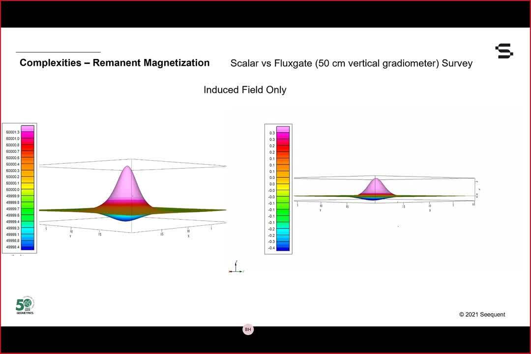
So now we’re going to show the modeled results
[00:16:17.330] 
from this target.
[00:16:18.270] 
And this first slide is,
[00:16:20.120] 
contains just the induced magnetic field.
[00:16:23.820] 
On the left-hand side we have the model data
[00:16:26.780] 
from the object as measured by a total field sensor.
[00:16:31.330] 
And on the right hand side,
[00:16:32.690] 
we have the model data as measured
[00:16:35.770] 
as would be measured from a gradient sensor
[00:16:39.510] 
with 50 centimeter with, on a gradient.
[00:16:45.180] 
This first slide shows just the induced field only.
[00:16:50.150] 
And as you can see, we have a large peak
[00:16:53.110] 
that’s to the Northeast of the
[00:16:58.420] 
target and a smaller trough to the south west.
[00:17:10.050] 
The next animation shows what happens
[00:17:13.450] 
when we have a remanent field that is the same amplitude
[00:17:17.940] 
as the induced magnetic field,
[00:17:20.940] 
and it’s oriented vertically downwards.
[00:17:22.830] 
As you can see,
[00:17:23.740] 
it changes the shape of the anomalies significantly,
[00:17:28.010] 
and we have a much larger trough
[00:17:30.490] 
now that’s still oriented towards the Southwest
[00:17:34.040] 
and it’s decreased the peak.
[00:17:38.520] 
All right, the third animation shows what happens
[00:17:41.880] 
when we have a remanent magnetization
[00:17:45.070] 
still the same amplitude, but now it’s oriented in the,
[00:17:50.120] 
towards the west horizontally.
[00:17:52.400] 
And as you can see it all,
[00:17:54.480] 
again, change the shape of the anomaly
[00:17:56.460] 
and now our smaller trough
[00:17:59.300] 
is oriented towards the Southeast.
[00:18:03.320] 
So this is quite a change from the original induced
[00:18:07.465] 
all the measurement that we have.
[00:18:11.060] 
The final animation in this slide
[00:18:13.500] 
is with the induced or the remanent field
[00:18:18.140] 
oriented towards the west.
[00:18:23.320] 
And as you can see this looks actually
[00:18:25.410] 
kind of similar to what we had with just the induced field,
[00:18:29.190] 
except now that the trough is oriented
[00:18:32.880] 
towards the Northwest.
[00:18:37.080] 
This just shows you some of the complexities
[00:18:39.440] 
that can arise when you have strong remanent magnetization,
[00:18:43.150] 
and it can distinctly change the shape of your anomaly
[00:18:46.360] 
and may cause you to misinterpret what you have.
[00:18:51.760] 
The next set of animations we’re going to model
[00:18:54.350] 
is using the same object
[00:18:56.760] 
and the same induced magnetization field,
[00:18:59.588] 
and use the same set of four parameters
[00:19:03.250] 
for the remanent magnetization.
[00:19:05.440] 
But what we’re doing, what we’ve done now
[00:19:07.910] 
is added noise that you’ll typically see
[00:19:10.470] 
from a total field survey and from a gradient survey
[00:19:14.600] 
so you can see how the remanent magnetization
[00:19:18.020] 
will change possibly the interpretation of the anomaly.
[00:19:22.320] 
The first animation is with the induced magnetic field only,
[00:19:27.710] 
and you can see the object quite well.
[00:19:31.640] 
The next animation has remanent magnetization
[00:19:35.780] 
that is oriented vertically downwards.
[00:19:40.440] 
The third animation has the remanent magnetization
[00:19:44.673] 
that is horizontal, but it’s in the Southern direction.
[00:19:48.933] 
And the final animation has the remanent magnetic field
[00:19:53.171] 
oriented horizontally but pointing to the west.
[00:19:57.840] 
And as you can see from our examples with noise,
[00:20:00.330] 
in some cases, the remanent magnetization
[00:20:03.200] 
can make an anomaly from a very metallic object
[00:20:06.640] 
look quite different than what you’re expecting
[00:20:08.970] 
from just an induced field anomaly.
[00:20:12.660] 
And in many cases that may lead you
[00:20:16.130] 
to not selecting the object as an object of interest
[00:20:21.660] 
or misinterpreting what that object is.
[00:20:26.184] 
We’re now going to discuss
[00:20:27.370] 
some of the different types of measurements
[00:20:29.340] 
that Stefan discussed in the introduction.
[00:20:33.640] 
We’re going to talk about two,
[00:20:35.250] 
basically two kinds of measurements.
[00:20:37.020] 
The first one is what we call a total field sensor,
[00:20:40.680] 
which measures just the magnitude of the field
[00:20:45.270] 
in, at a point in and time.
[00:20:49.010] 
These total field measurements
[00:20:50.470] 
are called total field sensors, scalar magnetometers,
[00:20:54.220] 
or atomic magnetometers.
[00:20:57.290] 
And then we’re also going to look at
[00:20:58.970] 
what are called gradient measurements.
[00:21:01.590] 
And what they look at is the difference
[00:21:03.800] 
in the magnetic field over a distance
[00:21:07.560] 
in a specific orientation.
[00:21:10.490] 
In most cases, gradient measurements are made with
[00:21:14.020] 
in either the vertical or a horizontal plane.
[00:21:18.640] 
With vertical gradient measurements,
[00:21:20.700] 
we measure the difference in the magnetic field
[00:21:23.560] 
from the top and the bottom of your sensor or sensor array.
[00:21:29.160] 
For horizontal gradient measurements,
[00:21:31.510] 
you’re looking at the difference across the width
[00:21:34.450] 
of your sensor or sensors array.
[00:21:38.300] 
Gradient measurements can be made with total field sensors
[00:21:41.930] 
that are separated
[00:21:43.480] 
by a specified distance, or they can be made
[00:21:46.060] 
with what are referred to as fluxgate sensors.
[00:21:51.200] 
On the left-hand side, we have a measurement
[00:21:53.280] 
that’s made by a fluxgate magnetometer
[00:21:55.720] 
in this case, the FM18.
[00:21:58.740] 
And this was done over the NSGG test site located in the UK.
[00:22:05.500] 
You can see various features on this map.
[00:22:08.280] 
And in particular,
[00:22:09.460] 
you can see clearly distinct anomalies
[00:22:12.370] 
to the, in the central Northern part of the map
[00:22:16.110] 
that were buried objects as tests for anomaly detection.
[00:22:21.720] 
And that’s shown on the left-hand side.
[00:22:25.260] 
On the right hand side,
[00:22:27.010] 
we have measurements that were made using
[00:22:30.140] 
two total field sensors separated by about a meter.
[00:22:34.860] 
And you can see the two maps are quite similar.
[00:22:37.660] 
There’s some differences.
[00:22:39.730] 
But in general, you can see the anomalies quite well.
[00:22:43.640] 
And it’s fairly easy to pick out our objects of interest.
[00:22:49.800] 
In the next slide, what we’re showing
[00:22:51.730] 
is the total field measurement made by a single sensor
[00:22:56.020] 
from the array of G858.
[00:22:58.530] 
And you can see this map looks different
[00:23:01.320] 
than the other sensors or other maps that we were showing.
[00:23:05.900] 
You can clearly see some of the large anomalies
[00:23:09.540] 
in the Northern half of this map,
[00:23:13.200] 
which were the buried objects.
[00:23:15.200] 
And you can see some other anomalies outside that region,
[00:23:18.900] 
but they tend to be a little bit more subtler.
[00:23:21.620] 
And that’s likely due to the fact
[00:23:23.540] 
that they were smaller objects nearer to the center
[00:23:27.880] 
or near to the surface.
[00:23:29.870] 
And in general these are not picked up as easily as
[00:23:35.620] 
the gradient measurements too.
[00:23:37.620] 
But, this map I would say tends to be a little bit
[00:23:42.130] 
less noisy.
[00:23:44.420] 
Where there are no objects
[00:23:46.070] 
you don’t see much magnetic field variation.
[00:23:49.380] 
The other thing you’ll note about this odd map is that
[00:23:53.010] 
there is a gradient, a long wavelength gradient
[00:23:59.748] 
in the data with the magnetic field decreasing
[00:24:02.200] 
to the south of this area
[00:24:05.260] 
that you did not see in a gradient field measurement.
[00:24:08.380] 
And this is because when you take two sensors
[00:24:12.380] 
or you’re just measuring the difference between two points,
[00:24:17.482] 
they will see the same long wavelength gradient
[00:24:21.090] 
and when you subtract out the field from the top and bottom,
[00:24:26.500] 
then there is no long-term wavelength difference
[00:24:31.020] 
in the measurement.
[00:24:32.750] 
So I just wanted to highlight that and I’ll just go in,
[00:24:37.300] 
in the next slide.
[00:24:39.100] 
So in this slide, I’ll discuss some of the reasons why
[00:24:42.760] 
there is a difference between measuring the magnetic field
[00:24:46.480] 
with a total field sensor or a scaler sensor
[00:24:49.920] 
versus a gradient sensor.
[00:24:54.570] 
The total field signal decreases in amplitude
[00:24:59.830] 
by a factor of one over R to the third with distance.
[00:25:05.890] 
The gradient signal decreases
[00:25:08.210] 
by a factor of one over R to the fourth.
[00:25:11.210] 
On the chart, on the right hand side,
[00:25:14.580] 
the decrease in amplitude is,
[00:25:18.440] 
with distance is represented by this blue curve
[00:25:22.780] 
for a total field measurement
[00:25:24.520] 
and a decrease in amplitude of the measurement
[00:25:27.580] 
for a gradient signal is shown in the red curve.
[00:25:33.790] 
And this distance and amplitude are normalized
[00:25:37.140] 
by the amplitude of the anomaly
[00:25:39.900] 
and also the length of the dipole.
[00:25:43.690] 
But as you can see at a factor,
[00:25:46.170] 
a distance of eight compared to the length of the dipole,
[00:25:51.160] 
the total field measurement in blue
[00:25:54.010] 
is actually an order of magnitude almost greater
[00:25:58.450] 
than the amplitude of the gradient measurement.
[00:26:05.750] 
And so this has a pretty big impact on your ability
[00:26:10.760] 
to detect objects at a greater range from your sensor.
[00:26:16.240] 
So in general, a total field measurement
[00:26:19.130] 
is more effective at detecting objects at greater distances.
[00:26:24.710] 
But, there are some advantages
[00:26:27.610] 
to doing gradient measurements.
[00:26:29.560] 
They tend to filter out low frequency trends
[00:26:31.910] 
as you saw in your previous map.
[00:26:34.530] 
The anomaly that you see from a gradient measurement
[00:26:37.810] 
is sometimes a little bit better defined.
[00:26:40.980] 
It’s sharper and narrower in width
[00:26:43.570] 
which makes it easier to determine the location
[00:26:47.560] 
of an object.
[00:26:50.700] 
And if you’re interested in shallow objects,
[00:26:54.860] 
it can also enhance the location and detection ability
[00:26:58.220] 
of those shallow objects.
[00:27:00.750] 
One other factor to consider
[00:27:02.280] 
when you look at gradient measurements
[00:27:04.150] 
is that they tend to be noisier.
[00:27:07.537] 
That’s because we’re actually taking the derivative
[00:27:10.160] 
of the magnetic field in that particular orientation,
[00:27:14.390] 
either vertically or horizontally
[00:27:16.670] 
and in all cases derivative measurements
[00:27:20.020] 
tend to act as a high pass filter.
[00:27:22.510] 
And noise in most magnetic surveys is,
[00:27:26.950] 
increases with frequency
[00:27:29.411] 
and so you will tend to increase noise
[00:27:34.160] 
in your measured signals.
[00:27:36.930] 
So, as a question I’d like to ask people,
[00:27:40.230] 
what kind of measurement the magnetic field measurements
[00:27:43.620] 
they have made in the past or plan to in the future.
[00:27:48.050] 
Do you use a total field sensor or atomic sensor,
[00:27:53.535] 
a gradient sensor such as a fluxgate
[00:27:55.760] 
or use a gradient array of total field sensors?
[00:28:00.420] 
Have you done both kinds of surveys
[00:28:02.280] 
or are you brand new to magnetic surveying
[00:28:05.170] 
and haven’t done anything?
[00:28:06.790] 
So please answer the poll in the chat window
[00:28:10.150] 
and we can discuss the results later on.
[00:28:32.960] 
Well, that concludes my section of the talk.
[00:28:35.560] 
And now I’m going to hand off the presentation
[00:28:37.880] 
to Becky Bodger from Seequent.
[00:28:40.870] 
I will be back to discuss the conclusions of this webinar,
[00:28:45.040] 
and also to answer any questions that you may have.
[00:28:49.837] 
<encoded_tag_open />v Becky<encoded_tag_closed />Thanks, Bart.<encoded_tag_open />/v<encoded_tag_closed />
[00:28:51.110] 
As mentioned, my name is Becky Bodger
[00:28:52.730] 
and I’m a geoscientist at Seequent.
[00:28:55.960] 
In this next section
[00:28:56.793] 
I’m going to show you a series of examples
[00:28:58.690] 
that were created using the forward modeling capabilities
[00:29:01.660] 
available in Oasis montaj with the UXO extension.
[00:29:05.330] 
The grid on the left is the background that I used
[00:29:07.660] 
for the forward modeling.
[00:29:08.910] 
It’s from an actual UXO survey in the North Sea,
[00:29:12.220] 
and is representative of the type and level of noise
[00:29:15.050] 
you would get on a real survey.
[00:29:17.080] 
In most of the examples,
[00:29:18.370] 
I’m using a 155 millimeter projectile
[00:29:21.700] 
unless otherwise stated.
[00:29:23.480] 
And there’s an image on the right
[00:29:25.840] 
that shows you what that looks like.
[00:29:31.880] 
So whenever you are working with any potential field data,
[00:29:34.880] 
for example, gravity or magnetics,
[00:29:37.000] 
we need to remember that mathematically
[00:29:38.840] 
magnetic anomalies are non-unique.
[00:29:40.940] 
Multiple theoretical solutions are possible.
[00:29:43.890] 
This is true whether we’re talking about geological features
[00:29:47.430] 
or anthropogenic objects.
[00:29:50.480] 
I found this image in a paper online
[00:29:52.400] 
that talks about the ambiguity in potential field modeling.
[00:29:55.800] 
And I like it because it demonstrates
[00:29:57.390] 
that the same Mickey mouse shaped deposit
[00:29:59.610] 
can have three different geophysical signatures.
[00:30:02.390] 
Why do we continue to use magnetics though,
[00:30:04.450] 
or any potential field data?
[00:30:06.190] 
Because there are ways to minimize this issue.
[00:30:10.760] 
So using a priori information in most cases
[00:30:13.660] 
especially when we were talking about anthropogenic objects,
[00:30:16.480] 
there’s history somewhere.
[00:30:18.720] 
If it’s UXO, we can research
[00:30:20.610] 
which munitions were dropped by either side
[00:30:23.130] 
during the various wars or conflicts.
[00:30:25.330] 
For archeology, hopefully you know some of the history
[00:30:28.100] 
of the area and what you are looking for,
[00:30:30.060] 
whether it’s an old burial site or building foundations.
[00:30:33.440] 
And for geotechnical investigations,
[00:30:35.660] 
there are often existing infrastructure maps
[00:30:37.980] 
showing the locations of buried cables and pipelines.
[00:30:41.290] 
This information is not always available,
[00:30:43.470] 
or it can be difficult to unearth,
[00:30:45.320] 
but it’s worth checking what’s available
[00:30:47.190] 
to aiding your processing and interpretation of the data
[00:30:50.050] 
before you start.
[00:30:53.780] 
Cross-referencing multiple types of geophysical data.
[00:30:57.450] 
So in the case of offshore geophysical surveys,
[00:31:00.500] 
mag is only part of the story.
[00:31:02.410] 
Oftentimes surveyors will simultaneously
[00:31:05.400] 
be collecting multi-team data, side scan, sonar,
[00:31:08.650] 
seismic, sub-bottom profile data, or even seabed images.
[00:31:13.110] 
Using the results of all of this data
[00:31:15.260] 
will really help with processing
[00:31:17.470] 
and the interpretation of your results.
[00:31:20.240] 
And in archeological studies, for example,
[00:31:22.760] 
you might have gravity and resistivity as well.
[00:31:28.560] 
Finally, use your common sense and be smart.
[00:31:31.770] 
You’re going to use common sense, your education,
[00:31:34.320] 
your past experience, all of that,
[00:31:36.320] 
to apply logic and find the best interpretation.
[00:31:40.760] 
Here, I attempt to demonstrate
[00:31:42.390] 
the non uniqueness of this mag anomaly.
[00:31:44.710] 
While they are not identical,
[00:31:46.620] 
I hope that we can agree that they are similar enough
[00:31:48.840] 
to demonstrate the point.
[00:31:50.780] 
So on the left we have two UXOs.
[00:31:52.890] 
One is an 81 millimeter projectile
[00:31:54.970] 
at 2.5 meters below the sensor.
[00:31:57.400] 
And one is a two and three quarter inch rocket
[00:31:59.490] 
at two meters below the sensor.
[00:32:01.440] 
On the right, we have a single UXO,
[00:32:04.200] 
which is the 155 millimeter that we’ve been looking at
[00:32:07.560] 
at 3.5 meters.
[00:32:09.590] 
And you can see that on the left-hand side,
[00:32:13.929] 
you know, the inflection point
[00:32:15.550] 
between the dipole’s a little bit slanted.
[00:32:17.610] 
It’s a little smaller than the one on the right.
[00:32:20.230] 
If we look at the profile below the grid,
[00:32:22.320] 
we can see that in profile they’re even harder
[00:32:24.890] 
to distinguish the differences.
[00:32:26.780] 
They both have similar positive and negative peaks.
[00:32:30.730] 
And again, the real only difference that we see here
[00:32:33.250] 
is the width of the actual dipole.
[00:32:38.360] 
This example also demonstrates the importance
[00:32:40.710] 
of griding your data and not only interpreting the results
[00:32:44.650] 
in, along the profile.
[00:32:46.490] 
It’s important to visualize it in 2D space
[00:32:48.770] 
to really see the full picture.
[00:32:51.120] 
So here’s another question for you guys.
[00:32:53.521] 
Which inclination of an object
[00:32:55.990] 
produces the strongest amplitude
[00:32:58.020] 
whether it’s peak to peak of the dipole
[00:33:00.090] 
or a single peak amplitude?
[00:33:02.290] 
Do you think it’s A, vertical, B horizontal,
[00:33:04.990] 
or C inclined at 45 degrees?
[00:33:09.130] 
So I’ll give you a few seconds
[00:33:10.150] 
just to putting your answers and then we’ll carry on.
[00:33:26.060] 
In this example, I’m going to show you the response
[00:33:28.220] 
of the object at different inclinations.
[00:33:32.570] 
So on the right,
[00:33:34.210] 
the image is just to represent the orientation
[00:33:36.920] 
we didn’t actually model the UXO that you’re seeing.
[00:33:40.890] 
So you can see that when it’s horizontal,
[00:33:42.640] 
it’s a nice perfect dipole.
[00:33:45.350] 
When you add inclination,
[00:33:46.820] 
so on the example that we modeled here
[00:33:48.780] 
was inclined at 45 degrees.
[00:33:50.800] 
You can see that the negative trough
[00:33:52.910] 
becomes a lot less negative.
[00:33:55.630] 
And when it’s perfectly vertical,
[00:33:58.630] 
you can see that the negative disappears altogether
[00:34:01.850] 
and you’re left with a monopole.
[00:34:04.770] 
And again, just remember,
[00:34:05.890] 
we’re not modeling the size of the UXO in the image,
[00:34:08.550] 
it’s just there to show you that it’s vertical is possible
[00:34:11.780] 
especially in the marine environment.
[00:34:14.560] 
So what’s the answer to the question that I asked?
[00:34:17.500] 
Here we have the three responses along a profile
[00:34:20.140] 
through the center of the dipole.
[00:34:22.370] 
The first is the horizontal,
[00:34:24.240] 
and we can see that the peak to peak amplitude
[00:34:27.750] 
is 5.4 nanoteslas.
[00:34:31.410] 
The second one in the middle here,
[00:34:32.730] 
is the object inclined at 45 degrees
[00:34:35.830] 
and it has a peak to peak value of six nanoteslas.
[00:34:39.600] 
And the vertical object has a positive monopole
[00:34:46.140] 
total peak value of 6.4 nanoteslas.
[00:34:50.600] 
So the answer to that last question was C for vertical.
[00:34:57.420] 
Next, we’re going to look at how the response changes
[00:35:00.170] 
as the object changes direction or destination.
[00:35:03.560] 
The top row is the horizontal 155 millimeter projectile
[00:35:07.721] 
at four meters below the sensor.
[00:35:10.640] 
And the bottom row is the inclined object at 45 degrees.
[00:35:15.600] 
Note how the negative part of the dipole
[00:35:17.490] 
decreases more rapidly as we rotate the inclined object.
[00:35:22.430] 
The first row is the near vertical object
[00:35:25.090] 
inclined at 85 degrees.
[00:35:26.930] 
And the second row is the same object
[00:35:29.960] 
inclined at negative 60 degrees
[00:35:33.580] 
which implies the opposite polarity.
[00:35:36.240] 
So, instead of the north pole up in the air,
[00:35:40.140] 
in this example, the south pole is up in the air.
[00:35:45.938] 
An interesting effect in the negative 60 degree example
[00:35:50.040] 
is also the halo that we see around the more obvious dipole.
[00:35:54.120] 
This is important
[00:35:55.130] 
when trying to model the depth of the object,
[00:35:57.783] 
whether you are using Euler deconvolution
[00:36:00.770] 
or an inversion style modeling method.
[00:36:03.540] 
Most methods require you to define the modeling window
[00:36:06.810] 
in order to select which data to invert.
[00:36:09.390] 
Since all of these examples use the exact same background
[00:36:12.600] 
which you can see in the top right-hand corner here,
[00:36:15.270] 
any differences in color that we see
[00:36:17.840] 
is part of the signal from the object.
[00:36:20.220] 
So for accurate modeling, we would ideally want to include
[00:36:23.060] 
as much of that signal as possible,
[00:36:25.130] 
which means it would require a much larger modeling window.
[00:36:30.400] 
Let’s also consider the effect of depth below the sensor
[00:36:34.090] 
on the inclined examples.
[00:36:35.840] 
So in the top row, we have the eastward facing
[00:36:38.560] 
155 millimeter projectile inclined at negative 60.
[00:36:42.750] 
And on the bottom, we have the same size projectile,
[00:36:45.020] 
but inclined at 45 degrees.
[00:36:47.170] 
And we can see the different response we get
[00:36:49.580] 
at 1.5 meters below the sensor, 2.5, 3.5, 4.5.
[00:36:55.780] 
And we can see that, we can actually see
[00:36:58.200] 
that none of these examples really produce
[00:37:00.010] 
that perfect looking dipole.
[00:37:01.920] 
And in fact, as the distance between the sensor
[00:37:04.400] 
and the object increases depending on the example,
[00:37:07.680] 
the positive in the top example
[00:37:09.420] 
and the negative in the bottom example,
[00:37:11.450] 
disappears almost entirely
[00:37:13.100] 
and leaves us with another parent monopole.
[00:37:17.500] 
So the last example or complexity
[00:37:19.710] 
I wanted to talk about today
[00:37:21.450] 
is simply the difficulty that arises
[00:37:23.370] 
when you have multiple objects stacked on top
[00:37:26.260] 
or close to one another.
[00:37:27.660] 
And this is a common phenomenon in test ranges
[00:37:30.770] 
or munition dumpsites.
[00:37:32.460] 
So on the left, I’ve modeled two UXOs.
[00:37:35.060] 
One is a 105 millimeter projectile
[00:37:37.540] 
at 3.5 meters below the sensor.
[00:37:40.650] 
Southward facing.
[00:37:42.210] 
And one meter away is a second UXO,
[00:37:45.133] 
a 60 millimeter projectile at two meters below the sensor
[00:37:48.180] 
and westward facing.
[00:37:50.360] 
It creates what I think would be called a complex dipole.
[00:37:54.310] 
On the right-hand side, is another example.
[00:37:56.510] 
A 155 millimeter at four meters
[00:37:59.080] 
and a 105 millimeters at two meter depth below sensor.
[00:38:03.170] 
Both roughly southward facing.
[00:38:05.200] 
With careful analysis, the example on the right
[00:38:08.100] 
could probably be accurately classified
[00:38:10.300] 
as two separate targets,
[00:38:12.340] 
but the example on the left would be a lot,
[00:38:15.300] 
would be much more difficult to separate.
[00:38:19.000] 
And I just wanted to give you a few,
[00:38:20.420] 
a couple of examples where we see this in real life
[00:38:23.330] 
and which caused a lot of problems.
[00:38:25.270] 
So in this example, this is a map
[00:38:27.450] 
of Lac Saint-Pierre in Canada.
[00:38:30.730] 
And I just wanted to show you the complexity
[00:38:32.470] 
and the problem that they’re dealing with here.
[00:38:34.950] 
And as an example, one of these large blue circles is,
[00:38:39.950] 
there are over 200 UXOs in that tiny little space.
[00:38:44.720] 
Another example in Europe is,
[00:38:47.820] 
this is the port in marked munition dump
[00:38:49.850] 
off the coast of Zeebrugge Harbor.
[00:38:52.190] 
This site contains a mix of world war I
[00:38:54.520] 
and world war II munitions,
[00:38:55.940] 
as well as a number of shipwrecks.
[00:38:58.050] 
This is a preliminary magnetic anomaly map.
[00:39:00.790] 
But now the real work begin is trying to separate the signal
[00:39:04.130] 
and finding the best method for cleaning up
[00:39:06.290] 
and monitoring the site.
[00:39:07.890] 
Because in these examples,
[00:39:09.680] 
mag alone will not get the job done.
[00:39:11.550] 
And you’ll, they’ll definitely need to use mag
[00:39:13.960] 
along with other geophysical methods to solve this problem.
[00:39:22.090] 
<encoded_tag_open />v Bart<encoded_tag_closed />In this section I talked about,<encoded_tag_open />/v<encoded_tag_closed />
[00:39:23.420] 
we talked about two factors that can influence
[00:39:26.063] 
the magnetic data that you measure.
[00:39:28.730] 
One is the remanent magnetization
[00:39:30.580] 
that can occur in ferromagnetic objects.
[00:39:33.320] 
And what we saw is that the presence
[00:39:35.750] 
orientation and strength of remanent magnetization
[00:39:39.838] 
can have a very strong impact
[00:39:41.970] 
on the anomaly amplitude in shape,
[00:39:44.800] 
and that it can be quite common in ferrous materials.
[00:39:49.200] 
And that’s sort of highlighted in these two images
[00:39:52.610] 
on the left-hand side of this slide.
[00:39:55.440] 
The other thing I discussed is the difference
[00:39:57.900] 
between a total field and gradient measurement
[00:40:01.130] 
of the magnetic field
[00:40:02.970] 
and how they differ and their ability to locate
[00:40:06.960] 
targets that are deeper
[00:40:08.210] 
or farther away from the sensor versus shallower,
[00:40:11.600] 
their noise levels and the impact
[00:40:14.950] 
of low frequency wavelength, spatial wavelengths signals
[00:40:19.340] 
on the data sets that you acquire.
[00:40:22.800] 
<encoded_tag_open />v Becky<encoded_tag_closed />So if there’s one key point<encoded_tag_open />/v<encoded_tag_closed />
[00:40:25.098] 
I’d like you to take away from my examples,
[00:40:26.660] 
it’s the presence of these monopoles.
[00:40:29.240] 
We always assume that the UXO
[00:40:31.300] 
is going to give us a nice clean dipole,
[00:40:33.330] 
and as we could see, that’s not the case.
[00:40:36.090] 
So, I mean, it was just a few minutes ago,
[00:40:38.130] 
but can you even remember all these examples
[00:40:40.660] 
that I showed you?
[00:40:41.810] 
So the first one, it was the
[00:40:43.680] 
155 inclined object at four meter depth.
[00:40:48.320] 
The next one was the 45 degree at 4.5 meter depth.
[00:40:54.930] 
This one was the 155 inclined at 85 degrees.
[00:41:01.710] 
So that’s almost vertical in the middle.
[00:41:03.720] 
And then this one was the negative 60 at four meters.
[00:41:07.630] 
So quite at a, quite a depth.
[00:41:10.220] 
And then that final one
[00:41:13.230] 
was the same negative 60 at 4.5 meters.
[00:41:18.600] 
So I think that was a really interesting
[00:41:21.155] 
observation from those examples.
[00:41:26.070] 
<encoded_tag_open />v Gretchen<encoded_tag_closed />Thank you again for joining us today.<encoded_tag_open />/v<encoded_tag_closed />
[00:41:28.710] 
If you have questions after this presentation,
[00:41:31.044] 
please feel free to email us
[00:41:32.930] 
at the address listed on the side.
[00:41:35.530] 
Don’t forget we will be having future webinars
[00:41:37.950] 
on magnetic data collection and magnetic data processing
[00:41:41.820] 
later on this year.
[00:41:43.660] 
We have not determined the dates for this yet,
[00:41:46.062] 
but we are tentatively scheduling them
[00:41:48.350] 
for November and December.
[00:41:51.150] 
We will be adding this recording
[00:41:52.760] 
to our Geometrics YouTube channel,
[00:41:54.700] 
and it will also be available on both
[00:41:56.800] 
the Seequent and Geometrics websites.
[00:42:00.370] 
Thank you again for your time
[00:42:01.660] 
and we hope our presentation was useful and informative.
<wpml_invalid_tag original=»PHA+» />[00:42:05.170] 
We look forward to hearing from you.

Магниторазведка антропогенных объектов: Теория

Это первый вебинар в серии из 3-х вебинаров по магниторазведке антропогенных объектов.

Смотреть больше видео по запросу

Узнайте больше об Oasis&nbsp;montaj

Расшифровка видеозаписи

Узнайте больше об Oasis montaj