Saiba como você pode visualizar, modelar e entender seus projetos ambientais criando e definindo plumas de contaminação usando as ferramentas geoestatísticas robustas da Extensão de contaminação para Leapfrog Works a fim de obter estimativas transparentes e defensáveis da massa e localização de contaminantes em seus projetos.

Este webinar abordará:

Uma introdução à Extensão de contaminação para Leapfrog Works.
O fluxo de trabalho de extensão Contaminants — com uma breve visão geral de:
Preparação e visualização de dados
Análise exploratória de dados e criação de domínios
Estimativa
Validação do modelo
Geração de relatórios
Sessão de perguntas e respostas ao vivo.

Visão geral

Palestrantes

Aaron Hollingsworth
Especialista em soluções para clientes da Seequent

Steve Law
Líder técnico sênior – Sequente

Duração

55 minutos

Veja mais vídeos sob demanda

Vídeos

Saiba mais sobre a solução para engenharia civil da Seequent

Saiba mais

Transcrição do vídeo

[00:00:00.320] 
<encoded_tag_open />v Aaron<encoded_tag_closed />So hello everyone<encoded_tag_open />/v<encoded_tag_closed /><!– wpml:html_fragment –>
[00:00:01.153] 
and welcome to today’s webinar
[00:00:02.400] 
on the Contaminants Extension for Leapfrog Works.
[00:00:05.990] 
Today we’ll be looking at the demonstration
[00:00:07.530] 
of the Contaminant Extension
[00:00:09.083] 
with time at the end of the webinar for your questions.
[00:00:12.460] 
My name is Aaron and I’m a Customer Solution Specialist
[00:00:15.540] 
here at Seequent, based in Brisbane office
[00:00:17.980] 
and I’m joined today by Steve Law
[00:00:19.710] 
our Senior Technical Lead for Geology.
[00:00:21.850] 
<encoded_tag_open />v Steve<encoded_tag_closed />Hello, I’m Steve<encoded_tag_open />/v<encoded_tag_closed />
[00:00:22.850] 
and I’m a Senior Technical Lead
[00:00:24.520] 
and I’m based here in (mumbles).
[00:00:30.180] 
<encoded_tag_open />v Aaron<encoded_tag_closed />Today we’ll first go through<encoded_tag_open />/v<encoded_tag_closed />
[00:00:31.280] 
a bit of background on Seequent
[00:00:32.680] 
and the Contaminants Extension.
[00:00:34.900] 
I’ll then hand over to Steve who will take us through
[00:00:37.680] 
the Contaminant Extension in Leapfrog Works itself.
[00:00:41.610] 
After that we’ll go through any questions that anyone has.
[00:00:44.240] 
So please if you do have any at any time,
[00:00:46.470] 
put them in here at the question or the chat window
[00:00:48.890] 
and go to webinar and we’ll get to them.
[00:00:53.604] 
There’s some background on Seequent.
[00:00:56.070] 
We are a global leader
[00:00:57.230] 
in the development of visual data science software
[00:00:59.470] 
and collaborative technologies.
[00:01:01.560] 
With our software you can turn complex data
[00:01:03.610] 
into geological understanding, providing timely insights
[00:01:07.220] 
and give decision makers confidence.
[00:01:10.270] 
At Seequent, our mission is to enable our customers
[00:01:12.640] 
to make better decisions about their earth
[00:01:14.590] 
and environmental challenges.
[00:01:18.430] 
The origins of Seequent go back to the 1990s
[00:01:21.570] 
when some smart people
[00:01:22.680] 
at the University of Canterbury in New Zealand,
[00:01:24.720] 
created the fast radio basis functions
[00:01:27.170] 
for efficiently generating 3D surfaces from point data.
[00:01:31.460] 
One of the applications that was seen for this
[00:01:33.300] 
was a better way to build geological modeling.
[00:01:36.080] 
And so in 2004, the company ARANZ Geo was founded
[00:01:39.490] 
and the Leapfrog software was first released
[00:01:41.680] 
to the mining industry.
[00:01:44.250] 
Since then the company has grown and evolved
[00:01:46.580] 
entering different industries
[00:01:48.240] 
such as geothermal energy, environmental and civil.
[00:01:52.960] 
And in 2017, ARANZ Geo rebranded to Seequent.
[00:01:58.000] 
In 2018, Seequent acquired Geosoft
[00:02:00.670] 
the developers of Geophysical Software
[00:02:02.520] 
such as a Oasis montaj.
[00:02:04.520] 
And then in 2019, acquired GeoStudio,
[00:02:07.710] 
the developers of Geotechnical Analysis Software.
[00:02:11.930] 
During this time Seequent has continued developing
[00:02:15.630] 
our 3D geological modeling in Leapfrog
[00:02:18.620] 
and collaboration tools such as Central.
[00:02:22.480] 
Earlier this year,
[00:02:23.313] 
Seequent was acquired by Bentley Systems
[00:02:25.940] 
and has become a Bentley company
[00:02:27.433] 
which opens us up to even more possibilities
[00:02:30.430] 
for future development for geoscience solutions.
[00:02:36.310] 
Seequent have office globally
[00:02:37.990] 
with our head office in Christchurch, New Zealand.
[00:02:40.890] 
And more locally we have offices in Australia,
[00:02:43.550] 
in Perth and in Brisbane.
[00:02:48.240] 
Like I mentioned Seequent’s involved
[00:02:49.970] 
in number of different industries
[00:02:52.140] 
covering things from a contaminant modeling,
[00:02:55.550] 
road and toll construction,
[00:02:57.360] 
groundwater detection and management,
[00:02:59.460] 
geothermal exploration, resource evaluation
[00:03:02.560] 
and so much more.
[00:03:08.210] 
Today we’re looking at contaminant
[00:03:10.253] 
or contaminated and environmental projects.
[00:03:13.340] 
Seequent provides solutions across the life
[00:03:15.650] 
of contaminated site projects
[00:03:17.060] 
from the initial desk study phase
[00:03:19.140] 
to the site investigation
[00:03:20.800] 
through to the remediation, design and execution.
[00:03:25.070] 
These solutions include our geophysics software
[00:03:27.320] 
such as Oasis montaj and VOXI.
[00:03:29.930] 
Our 3D visualization and geological modeling
[00:03:32.490] 
and contaminant modeling in Leapfrog Works
[00:03:35.460] 
as well as flow and transport analysis in GeoStudio.
[00:03:39.710] 
Across all of this we have Seequent Central
[00:03:42.100] 
a cloud-based model management and collaboration tool
[00:03:45.320] 
for the life of the projects.
[00:03:48.090] 
Like I said, today we’re specifically looking
[00:03:50.220] 
at the Contaminants Extension in Leapfrog Works.
[00:03:56.040] 
So what is the Contaminants Extension?
[00:03:58.670] 
The Contaminants Extension
[00:03:59.790] 
is an optional module for Leapfrog works
[00:04:01.660] 
to enable spatial modeling of numeric data
[00:04:04.540] 
for defining the concentration, distribution
[00:04:07.330] 
and mass of the institute contamination at a site.
[00:04:11.910] 
The Seequent Contaminants Extension provides
[00:04:14.670] 
a transparent and auditable data-driven interpretation.
[00:04:19.900] 
It provides interactive visual tools
[00:04:22.430] 
with the extension that makes geostatistics
[00:04:24.760] 
accessible for all geoscientists
[00:04:27.610] 
ensuring that you and your teams
[00:04:29.120] 
can work the best with your data.
[00:04:32.600] 
It has built-in report tables
[00:04:34.730] 
and cross-section evaluations
[00:04:36.270] 
that are dynamically linked
[00:04:37.620] 
to your plume models and your data.
[00:04:41.350] 
So they will update automatically
[00:04:43.430] 
as the investigation and the project evolves in new day
[00:04:47.010] 
that comes into your Leapfrog project.
[00:04:50.320] 
It also means there’s an interrogatable estimation tool
[00:04:54.730] 
that provides easy access to the details
[00:04:58.260] 
for how you’ve created your informed decisions.
[00:05:02.595] 
In short, it allows you to take known data for your project
[00:05:07.070] 
and analyze it with spatial variability
[00:05:09.500] 
of the concentrations for your data
[00:05:12.390] 
and it helps you define your projects.
[00:05:20.860] 
So that’s what it is.
[00:05:22.410] 
Why did we develop it? And why is it useful?
[00:05:25.800] 
Well, we did it because we wanted to provide
[00:05:27.840] 
these accessible best practice solution tools
[00:05:30.690] 
for you to model your contamination plumes.
[00:05:34.290] 
We wanted to make characterizing contaminated land
[00:05:36.810] 
in groundwater, in a rigorous and auditable way
[00:05:39.730] 
that combines 3D dynamic geological Models
[00:05:42.700] 
with these best practice geostatistical methods.
[00:05:47.500] 
The ultimate goal of estimation
[00:05:48.970] 
is to combine the qualitative geological interpretation
[00:05:52.310] 
of your project.
[00:05:53.680] 
So your geological models
[00:05:55.270] 
with the sparsely sampled quantitative data
[00:05:58.450] 
to create spatial predictions
[00:06:00.130] 
for the distribution of that contaminant plan.
[00:06:09.140] 
The Contaminants Extension
[00:06:10.610] 
coupled with Seequent Central provides a wholistic way
[00:06:13.877] 
for the engineer and modeler for a project
[00:06:16.780] 
to effectively understand
[00:06:18.580] 
and importantly communicate the site conditions
[00:06:21.490] 
with both internal and external stakeholders
[00:06:24.310] 
in a collaborative environment.
[00:06:27.090] 
The graphic here shows an overview of the flow
[00:06:29.610] 
from Leapfrog to Central as part of the solution.
[00:06:34.350] 
Starting at the base here and moving up
[00:06:37.690] 
we can see that with your investigation data models
[00:06:40.982] 
and estimations can be created by the modeler
[00:06:44.260] 
and the environmental engineer for instance.
[00:06:48.310] 
And using Central,
[00:06:49.600] 
they can share this and collaborate on this
[00:06:53.000] 
with internal team members such as managers,
[00:06:55.830] 
reviewers or other modelers
[00:06:58.360] 
to build up the understanding of the site
[00:07:02.040] 
or as part of the project review process.
[00:07:06.420] 
At the very top of this infographic here
[00:07:08.260] 
we can then see how we can use Central
[00:07:10.330] 
to engage with external stakeholders
[00:07:13.130] 
such as the clients or other contractors
[00:07:16.650] 
and you can bring them into the Central project again
[00:07:18.740] 
to communicate in an interactive and visual way.
[00:07:24.820] 
The Seequent solution for the contaminant projects then
[00:07:27.490] 
is all about knowing the impact
[00:07:29.490] 
of environmental contamination for your projects.
[00:07:32.880] 
Through first seeing the problem
[00:07:34.360] 
in a clear, intuitive and visual way.
[00:07:38.030] 
The picture is worth 1,000 words
[00:07:39.440] 
a 3D visualization of the site has to be worth a million.
[00:07:44.260] 
With a Contaminants Extension,
[00:07:45.810] 
it’s an interactive dynamic site model
[00:07:47.990] 
you can create and understand
[00:07:50.130] 
and aid in your analysis and your assumptions
[00:07:53.070] 
and recommendations for your reports.
[00:08:01.340] 
I’ll now hand over to Steve
[00:08:03.500] 
who will take us through Leapfrog
[00:08:05.540] 
and the Contaminants Extension.
[00:08:27.267] 
So we’ll just switch over from the slides here. (mumbles).
[00:08:38.840] 
<encoded_tag_open />v Steve<encoded_tag_closed />Thanks very much Aaron<encoded_tag_open />/v<encoded_tag_closed />
[00:08:40.756] 
for that great introduction.
[00:08:42.290] 
So I’m going to go through the
[00:08:44.470] 
Contaminants Extension Workflow.
[00:08:48.830] 
The end result is a resource model
[00:08:50.820] 
and through the whole process we have a look at our data.
[00:08:53.770] 
We go through the mining,
[00:08:55.340] 
run through estimations and validate and report at the end.
[00:08:59.650] 
Throughout the whole process it’s not a linear
[00:09:01.960] 
it can be a cyclical process
[00:09:03.840] 
so that whilst we’re at any stage
[00:09:06.310] 
we can always go back to our geology
[00:09:08.480] 
and look at how things are relating to each other.
[00:09:15.580] 
We’re going to go through a couple of key steps
[00:09:18.950] 
that we need to consider whilst building up a plume model.
[00:09:24.070] 
So the first part is being well aware of our data
[00:09:27.960] 
and how we can visualize it very easily
[00:09:30.240] 
within Leapfrog Works.
[00:09:31.980] 
So we want to consider things,
[00:09:33.659] 
where is our data and how is it located especially?
[00:09:37.500] 
We have tools in-built that we can check
[00:09:39.640] 
and make sure our data is validated
[00:09:42.490] 
and we have really good visualization tools.
[00:09:47.360] 
So within this project we have three models,
[00:09:51.440] 
the first one is a geology model
[00:09:53.840] 
and you can see here that it’s got outwash
[00:09:59.580] 
and ice deposits until above a bedrock sequence.
[00:10:03.960] 
And within that we have a range of vertical boreholes
[00:10:07.210] 
and these have been sampled generally in isolated locations
[00:10:13.840] 
for a chlorine contaminant
[00:10:16.030] 
and that’s what we’re going to be evaluating.
[00:10:19.240] 
As well as the geology model,
[00:10:21.440] 
we have a water table model.
[00:10:24.870] 
And this has been divided into a saturated
[00:10:28.040] 
and made (mumbles) again above bedrock.
[00:10:31.740] 
So one of the first things we want to consider is,
[00:10:34.910] 
is there any specific way that we should domain our data?
[00:10:38.040] 
To ask some of them, is chlorine associated with pathology?
[00:10:42.960] 
Is it associated with water table or a combination of both?
[00:10:47.199] 
And we have some tools within Leapfrog Works
[00:10:49.460] 
that can show this.
[00:10:52.180] 
So up in the boreholes’ database here,
[00:10:55.010] 
I have a table with the contaminants
[00:11:00.320] 
and then I’ve got a geology table.
[00:11:02.370] 
We have a merge table function
[00:11:04.090] 
so I’ve been able to merge these together.
[00:11:06.370] 
And this enables me then to evaluate them
[00:11:10.700] 
using some statistical tools
[00:11:13.120] 
in this case I’m using a box plot.
[00:11:17.640] 
And so this was here as a box plot of the geology
[00:11:20.360] 
against the contaminant.
[00:11:22.610] 
And we can see here that that is telling me
[00:11:24.910] 
that the outwash and local ice to contact deposits
[00:11:28.310] 
and the two, have the highest concentration of chlorine.
[00:11:32.310] 
And then there’s a lot less amount
[00:11:34.350] 
in the outwash deposits and bedrock.
[00:11:38.830] 
We can also have a look at this as a table of statistics.
[00:11:48.536] 
Excuse me.
[00:11:58.460] 
An idea of…
[00:11:59.810] 
We have a little bit total concentration.
[00:12:02.200] 
I can see the actual values within each one.
[00:12:06.220] 
One of the key things here is
[00:12:07.510] 
looking at the number of samples
[00:12:09.010] 
so we have only two samples within the bedrock.
[00:12:12.060] 
We’d identified that the outwash and ice deposits
[00:12:14.920] 
and the two had the greatest concentrations
[00:12:20.080] 
and we’ve got the most number of samples in those as well
[00:12:22.650] 
so we’ve got approximately 70 samples within the ice.
[00:12:27.310] 
And we’ve got the mains
[00:12:28.780] 
so we’ve got much higher means within ice
[00:12:32.660] 
and very low within the outwash deposits
[00:12:35.760] 
and again quite low
[00:12:36.970] 
but there’s only two samples within bedrock.
[00:12:41.280] 
So in this instance there’s no clear
[00:12:46.220] 
if we have a look at (mumbles)
[00:12:49.820] 
water table, we can see that both are saturated
[00:12:54.180] 
and the vital sign has significant concentrations
[00:12:59.030] 
and there’s not one particularly higher than the other.
[00:13:01.610] 
Saturated is a little bit more,
[00:13:03.600] 
but it’s not obviously completely different.
[00:13:08.900] 
So the way we’ll consider this then
[00:13:10.870] 
is I’m just going to separate a single domain
[00:13:13.940] 
that’s above bedrock and not taking into account
[00:13:16.790] 
whether it’s saturated or (mumbles).
[00:13:20.030] 
In this way, I have a geological model then
[00:13:23.370] 
that is just domained.
[00:13:37.140] 
So, once we’ve decided on
[00:13:38.630] 
how we’re going to domain our data,
[00:13:40.620] 
then we start using the Contaminants Extension information
[00:13:43.990] 
and we can link it to our geology model
[00:13:46.040] 
right through to the resource estimate.
[00:13:48.060] 
And we can do exploratory data analysis
[00:13:50.400] 
specifically on the domain itself.
[00:13:53.635] 
So we have a look at the domain model.
[00:13:57.190] 
And in this case
[00:13:58.023] 
this has now been all of the mythologies about bedrock
[00:14:02.320] 
have been combined into a single domain
[00:14:03.660] 
which is the yellow one on the scene.
[00:14:06.370] 
And we can see that the majority of the samples
[00:14:08.147] 
are within that and there’s just the one isolated to
[00:14:12.140] 
below in the bedrock which we won’t be considering
[00:14:14.960] 
in this particular estimate.
[00:14:24.890] 
When we build up estimation,
[00:14:29.130] 
we have what’s termed as contaminants model folder.
[00:14:32.230] 
So when we activate the Contaminants Extension License,
[00:14:37.600] 
it displays up as a folder in your project tree
[00:14:41.380] 
and there’s a estimation sub folder
[00:14:43.347] 
and a block model’s folder.
[00:14:45.490] 
The estimation folder can be considered to be
[00:14:47.950] 
where you set up all your parameters.
[00:14:49.930] 
And then the block model is where we display
[00:14:52.500] 
all of our results
[00:14:53.440] 
and we also do all our reporting and validation
[00:14:56.140] 
from that point as well.
[00:14:58.520] 
So I’ve decided to do a title constraint traction
[00:15:02.410] 
of this chloride within the unconsolidated domain
[00:15:05.870] 
which is this yellow block here.
[00:15:08.010] 
So when we create a domain estimator,
[00:15:12.920] 
we just select any closed solid within our project
[00:15:17.040] 
and you can see here that
[00:15:17.890] 
this is the unconsolidated sediments
[00:15:21.430] 
within our domain model.
[00:15:24.160] 
And then the numeric values are coming directly
[00:15:26.940] 
from our essay table, contaminant intervals,
[00:15:30.681] 
total concentration.
[00:15:32.760] 
So we can choose any numeric column
[00:15:34.860] 
within any part of our database.
[00:15:36.860] 
And also if we were storing point data
[00:15:39.520] 
within the points folder over here,
[00:15:41.630] 
we would be able to access that as well.
[00:15:43.980] 
So it doesn’t have to be within drew holes .
[00:15:48.720] 
I’m not applying any transform at this stage
[00:15:51.680] 
and we also have the capability of doing compositing.
[00:15:55.340] 
This data set doesn’t render itself to compositing
[00:15:58.790] 
because it’s got isolated values within each holes
[00:16:02.640] 
really only got one or two samples
[00:16:05.628] 
compositing small for if we’ve got a
[00:16:08.080] 
continuous range of samples down the borehole,
[00:16:12.020] 
and we’d want to composite that into large intervals
[00:16:17.510] 
to reduce their variance.
[00:16:20.170] 
So within each estimation for each domain,
[00:16:22.730] 
we have this sub folder.
[00:16:24.520] 
And from there we can see the domain itself.
[00:16:28.280] 
So we can double check that that is the volume of interest
[00:16:33.030] 
and we can display the values within that domain.
[00:16:37.700] 
So they have become point values at this stage
[00:16:42.800] 
and you can label those
[00:16:44.820] 
and you can also do statistics on these.
[00:16:47.610] 
So these now become domain statistics.
[00:16:50.500] 
So by right clicking on the values,
[00:16:54.280] 
I get a histogram of those values there.
[00:16:58.910] 
As with all Leapfrog Works graphs,
[00:17:04.010] 
they are interacting with the 3D scene.
[00:17:07.130] 
So let’s just move this over here.
[00:17:12.920] 
If I wanted to find out where these core values were,
[00:17:17.590] 
I can just highlight the one that on the graph
[00:17:20.610] 
and that will show up in the same format.
[00:17:23.450] 
Let’s do these ones about 100, there they are there.
[00:17:27.350] 
So gives us then idea of whether or not
[00:17:30.160] 
we need to create sub domains.
[00:17:32.400] 
If all the high grades were focused a little bit more
[00:17:35.520] 
we might be able to subdivide them out.
[00:17:37.210] 
But in this case,
[00:17:38.630] 
we’re just going to treat everything in the one domain.
[00:17:44.870] 
The special models folder is where we can do variography
[00:17:49.990] 
which is a spatial analysis of the data
[00:17:52.670] 
to see whether there are any specific directions
[00:17:55.320] 
where the concentration grades might be aligned.
[00:18:02.980] 
I’ll open this one up.
[00:18:12.510] 
So the way the variography works
[00:18:14.320] 
is that we select the direction
[00:18:16.700] 
and then we model it in three directions.
[00:18:21.370] 
One with the greatest degree of continuity et cetera.
[00:18:25.160] 
This radio plot is a plane within this.
[00:18:29.390] 
We’re looking in a fairly horizontal plane here
[00:18:32.667] 
and you can see that we have…
[00:18:35.600] 
we can always see the ellipsoid that we’re working with
[00:18:38.900] 
so to see whether it’s in the like
[00:18:41.160] 
we wanted to make that a little bit flatter.
[00:18:43.250] 
We didn’t leave it in a 3D scene
[00:18:45.660] 
and it will update on the form here
[00:18:48.210] 
and the graphs will update.
[00:18:51.260] 
We can use this radial plot.
[00:18:54.520] 
This may suggest that this orientation
[00:18:57.210] 
has a little bit more continuity and we’ll re-adjust.
[00:19:02.520] 
This particular data set doesn’t create
[00:19:05.680] 
a very good experimental variogram
[00:19:08.130] 
so we do have some other options
[00:19:09.710] 
where we could use a log transform prior to that
[00:19:14.293] 
so here I’ve done a log transform on the values
[00:19:19.450] 
and that was simply done by at the very beginning.
[00:19:22.550] 
When I selected my samples
[00:19:24.256] 
I could apply a log transform in through here.
[00:19:28.630] 
This gets rid of some of the variability
[00:19:30.650] 
especially the range and extreme differences
[00:19:34.350] 
between very high values and very low values
[00:19:37.260] 
and this can help develop a better semi-variably model
[00:19:42.300] 
if we have a little bit this one.
[00:19:50.624] 
You can see here that the semivariogram
[00:19:53.240] 
is a little bit better structured than it was before.
[00:19:56.700] 
Again this data is quite sparse.
[00:19:58.760] 
So this is about the best we could do
[00:20:01.070] 
with this particular data set.
[00:20:04.090] 
We have the ability to pick a couple of range of structures,
[00:20:08.970] 
we have a nugget plus a potentially two structures
[00:20:12.370] 
but in this case I’ll just pick a nugget,
[00:20:15.360] 
a fairly large nugget and a single structure
[00:20:18.030] 
which is sufficient to model this.
[00:20:21.190] 
We can get an idea of that model.
[00:20:23.350] 
So this is in the…
[00:20:25.090] 
The range is quite large, 1200 to 1400 meters.
[00:20:29.920] 
And that’s because the data itself is quite widely spaced.
[00:20:33.620] 
And we’ve only got a very short range
[00:20:35.390] 
in the Z direction because we’re looking at a
[00:20:37.294] 
fairly constrained tabular body of potential contamination.
[00:20:44.340] 
The advantage to building the variography
[00:20:46.390] 
within the contaminants extension is that
[00:20:49.070] 
everything is self-contained,
[00:20:50.410] 
and once we hit the side button,
[00:20:52.830] 
then that variogram is all ready to use
[00:20:56.510] 
within the estimations itself.
[00:21:00.480] 
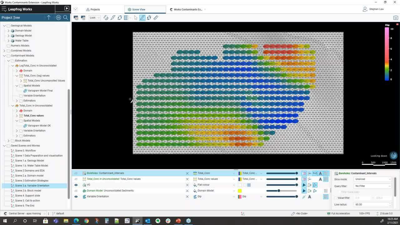
We also have a concept of variable orientation.
[00:21:04.750] 
Sometimes the design of the Contaminant
[00:21:10.520] 
isn’t purely tabular
[00:21:12.480] 
and there may be local irregularities
[00:21:14.810] 
within the surfaces.
[00:21:16.680] 
So we can use those surfaces
[00:21:18.450] 
to help guide the local orientation of the variogram
[00:21:22.750] 
when we’re doing sample selection.
[00:21:25.470] 
So just don’t want it here already.
[00:21:31.890] 
So the way we do that
[00:21:32.810] 
is that we set up a reference surface
[00:21:35.440] 
and in this case it’s the actual base
[00:21:37.570] 
over the top of the bedrock
[00:21:39.530] 
and we can see here that we’ve colored this by a dip.
[00:21:44.480] 
So we can see that we’ve got some varying dips
[00:21:47.670] 
that flat up in the middle
[00:21:49.070] 
and slightly more dips around the edges.
[00:21:51.830] 
If I can hop and look cross sections through there,
[00:22:03.450] 
we can see that what will happen
[00:22:06.610] 
is when we pick out samples,
[00:22:09.060] 
the ellipsoid will be orientated as local
[00:22:12.780] 
and so overall ellipsoid is in this general direction,
[00:22:16.010] 
but where it gets flat out,
[00:22:17.400] 
it will rotate in a flat orientation.
[00:22:21.570] 
The actual ratios and the variogram parameters themselves
[00:22:24.960] 
are still maintained.
[00:22:26.267] 
It’s just the orientation
[00:22:28.260] 
for when the samples are being selected.
[00:22:35.270] 
When we’re doing an estimation,
[00:22:36.730] 
we have to consider a few different things.
[00:22:39.330] 
So we need to understand what the stage our project is
[00:22:42.650] 
and this might help us work out
[00:22:44.520] 
which estimation method to use.
[00:22:46.550] 
If we’ve got early stage,
[00:22:48.190] 
we might not have very much data.
[00:22:49.910] 
We might not have sufficient data to get a variogram.
[00:22:52.740] 
So we will need to use either nearest neighbor
[00:22:55.510] 
or inverse distance type methods.
[00:22:59.476] 
There can be a lot of work to go into the search strategy.
[00:23:02.280] 
And that is how many samples are we going to use
[00:23:05.061] 
to define a local estimate.
[00:23:08.850] 
And then once we run our estimate,
[00:23:10.900] 
we need to validate it against the original data
[00:23:14.250] 
to make sure that we’re maintaining the same kind of means
[00:23:17.950] 
and then we want to report our results at the end.
[00:23:23.150] 
To set up the estimators,
[00:23:25.970] 
we work through this estimators sub folder here
[00:23:29.760] 
and if you right click
[00:23:30.920] 
you can go have inverse distance nearest neighbor kriging
[00:23:34.857] 
and we can do ordinary kriging, simple kriging
[00:23:38.010] 
or we can use the actual RBF estimator as well.
[00:23:41.520] 
Which can be quite good
[00:23:42.870] 
for when we haven’t got sufficient data to a variogram.
[00:23:47.110] 
It’s a global estimator.
[00:23:49.540] 
Using the same underlying algorithm
[00:23:51.470] 
that is used for when we krig the surfaces
[00:23:54.170] 
or the numeric models that can be run
[00:23:56.600] 
within Leapfrog Works itself.
[00:24:00.710] 
To set one up
[00:24:01.990] 
once I open we can edit that,
[00:24:04.650] 
we can apply clipping which is
[00:24:08.390] 
if we want to constrain the very high values
[00:24:11.010] 
and give them less influence,
[00:24:12.550] 
we can apply that on floor.
[00:24:15.090] 
In this case because I’ve actually looking at contaminants
[00:24:17.380] 
I don’t really want to cut them down initially
[00:24:19.580] 
so I will leave them unclicked.
[00:24:22.540] 
I’m just doing point kriging in this case
[00:24:24.710] 
so just I’m not using discretization at all.
[00:24:28.590] 
In some cases if I want to block kriging,
[00:24:30.460] 
then I would increase these discretization amounts.
[00:24:35.170] 
I’m using ordinary kriging.
[00:24:36.693] 
This is where we determine ordinary or simple.
[00:24:41.120] 
And this is the variogram.
[00:24:42.750] 
So you can pick.
[00:24:44.180] 
It will see the variogram within the folder.
[00:24:50.460] 
You set to a particular variogram
[00:24:53.090] 
and that’s more for making sure
[00:24:55.730] 
that it’s set to the correct orientation.
[00:24:58.240] 
And then it’ll automatically go to the maximum range
[00:25:01.100] 
of that variogram but you can modify these
[00:25:03.680] 
to be less than that or greater.
[00:25:05.790] 
Depends on the circumstances
[00:25:08.750] 
and often you’ll do a lot of testing
[00:25:11.230] 
and sensitivity analysis to determine
[00:25:13.760] 
the best scope for this one.
[00:25:18.400] 
And then we can choose
[00:25:19.890] 
minimum and maximum number of samples.
[00:25:22.610] 
And this effectively becomes
[00:25:24.280] 
our grade variable within the block model
[00:25:27.710] 
and we can store other variables as well.
[00:25:30.510] 
So if we’re using kriging,
[00:25:32.030] 
we can store things such as kriging variance,
[00:25:34.240] 
slope and regression
[00:25:35.820] 
which would go as to how good the estimate might be.
[00:25:39.430] 
We can store things such as average distance to samples
[00:25:42.290] 
and these may help us with classification
[00:25:44.810] 
criteria down the track.
[00:25:47.150] 
So I’ve created us an ordinary kriged estimator here
[00:25:52.640] 
and then I’ve also got one.
[00:25:54.270] 
This one is exactly the same,
[00:25:57.340] 
but in this case I’ve actually applied
[00:25:59.610] 
the variable orientation.
[00:26:01.230] 
So we’ve set up a variable orientation within the folder.
[00:26:04.190] 
It will be accessible in our parameter set up through here
[00:26:09.050] 
and I’ll give it a slightly different name.
[00:26:11.550] 
This one I will need to compare the kriging results
[00:26:17.310] 
with and without variable orientation apply.
[00:26:21.570] 
So we set up all of our different parameters
[00:26:24.250] 
in this estimation folder.
[00:26:27.360] 
And we are then able to create a block model
[00:26:32.690] 
to look at the results.
[00:26:40.300] 
Setting up a block model is quite simple
[00:26:43.440] 
so we can create a new block model
[00:26:45.900] 
and we can also import block models from other software.
[00:26:49.790] 
And when we’ve created one,
[00:26:51.990] 
we can edit it by opening it up.
[00:26:55.500] 
And in this case,
[00:26:56.333] 
we’ve got a block size of 80 by 80 meters
[00:26:58.720] 
in the X, Y direction and five in the Z
[00:27:02.260] 
so we’re looking at that fairly thin.
[00:27:04.270] 
And if we’re looking at it again very visual
[00:27:07.167] 
and we can see our block size.
[00:27:13.230] 
So this is 80 by 80 in the X Y direction here.
[00:27:18.400] 
And we can change these boundaries at any time.
[00:27:20.810] 
So once it’s been made,
[00:27:21.900] 
if we wanted to adjust it,
[00:27:23.533] 
I could just move the boundary up
[00:27:25.720] 
and it will automatically update the model.
[00:27:28.930] 
I want to do that now so it doesn’t rerun.
[00:27:31.820] 
A key concept when working with block models
[00:27:34.030] 
within the Contaminants Extension is this evaluations tab.
[00:27:38.260] 
So basically whatever we want to flag into the block model
[00:27:41.794] 
needs to come across from the left-hand side
[00:27:44.590] 
across to the right.
[00:27:46.040] 
So what I’m doing here
[00:27:47.090] 
is I’m flagging each block centroid with the domain model
[00:27:50.980] 
so that will flag it with whether it’s within that domain
[00:27:56.590] 
but we can also flag at geology.
[00:27:58.410] 
So this will put into whether it’s two
[00:28:00.770] 
or whether it’s bedrock
[00:28:02.610] 
and also avoid us saturated sides
[00:28:05.110] 
could be flagged as well.
[00:28:07.500] 
And then this is Y grade or contaminant variables here.
[00:28:12.870] 
So I’m just putting in all four that are generated
[00:28:17.200] 
so I’ve got an inverse distance,
[00:28:19.360] 
I’ve got two different krigings.
[00:28:21.734] 
And also the nearest neighbor.
[00:28:23.460] 
Nearest neighbor can be useful
[00:28:25.140] 
for helping with validation of the model.
[00:28:29.480] 
Again, any of these can be removed or added at one time.
[00:28:32.680] 
So if I did want to look at the RBF,
[00:28:35.070] 
I would just bring it across
[00:28:37.170] 
and then the model would rerun.
[00:28:41.200] 
So we can see here, the model has been generated.
[00:28:45.710] 
And one of the key things for validation of first
[00:28:49.120] 
is to actually look at the samples against the results.
[00:28:54.550] 
So if I just go into a cross section
[00:29:06.010] 
making sure that our color schemes
[00:29:08.760] 
forbides the data and the bot model are the same
[00:29:11.940] 
and we can import these colors
[00:29:13.580] 
so if we’ve got colors defined for our essays up here,
[00:29:23.952] 
we can export those colors
[00:29:25.640] 
like create a little file,
[00:29:27.360] 
and then we can go down to our block model
[00:29:29.660] 
and we can import those colors down here.
[00:29:34.420] 
So I did on this one, look at that colors import
[00:29:38.370] 
and then pick up that file.
[00:29:39.670] 
And that way we get exactly same color scheme.
[00:29:42.640] 
And what we’re hoping to see
[00:29:43.910] 
is a little we’ve got yellows
[00:29:46.610] 
we should hopefully have orange or yellows around,
[00:29:49.710] 
higher grades will be in the reds and purples
[00:29:53.610] 
and lower grades should show up.
[00:30:02.308] 
Of course we have a lot of data in here.
[00:30:06.074] 
There we go.
[00:30:06.907] 
So we can see some low grade points over here
[00:30:09.280] 
and that’s equating.
[00:30:11.170] 
We’ve got really good tools for looking at the details
[00:30:14.870] 
of the results on a block-by-block basis.
[00:30:17.720] 
If I highlighted this particular block here,
[00:30:21.250] 
we have this interrogate estimator function.
[00:30:26.130] 
And this is the estimator that it’s looking at.
[00:30:29.080] 
So like ordinary krig without variable orientation
[00:30:32.560] 
it’s found there’s many samples
[00:30:35.390] 
and depending on how we’ve set up our search,
[00:30:38.120] 
in this case it’s included all those samples.
[00:30:41.050] 
It’s showing us the kriging lights
[00:30:42.360] 
that have been applied and we can sort these
[00:30:45.177] 
and distances from the sample.
[00:30:48.660] 
So we can see the closest sample used was 175 meters away
[00:30:53.080] 
and the greatest one was over 1,000 meters away.
[00:30:56.200] 
But it’s got lights through there.
[00:31:00.470] 
Part of the kriging process
[00:31:01.730] 
can give negative kriging weights
[00:31:03.670] 
and that is not a problem
[00:31:04.850] 
unless we start to see negative grade values.
[00:31:07.770] 
In that case, you might need to change
[00:31:09.520] 
our sample selection a little bit
[00:31:12.660] 
to eradicate that influence.
[00:31:16.420] 
That’s just part of the kriging process.
[00:31:21.130] 
You can see also that when we do that we can…
[00:31:23.740] 
it shows the ellipsoid for that area.
[00:31:26.720] 
And if we filter the block model
[00:31:30.818] 
and I’ll just take away the ellipsoid for a second,
[00:31:36.180] 
it shows you the block and it shows you the samples
[00:31:39.113] 
that are being used.
[00:31:40.540] 
So you’ve got a nice spatial visualization
[00:31:44.000] 
of what samples are actually being used
[00:31:46.080] 
to estimate the grade within that box through there.
[00:31:48.947] 
And if you want to try something else,
[00:31:50.760] 
you can go directly to the estimator and modify.
[00:31:55.360] 
If I want to change this to three samples,
[00:31:58.070] 
reduce these chains to search
[00:32:00.600] 
and you can get see what the impacts could be. Okay.
[00:32:06.790] 
So apart from visualization
[00:32:08.910] 
and looking at on a block-by-block basis,
[00:32:12.620] 
we can also run swath plots.
[00:32:18.780] 
So within the block model itself,
[00:32:20.870] 
we can create a new swath plot.
[00:32:23.210] 
And the beauty of this is that
[00:32:25.200] 
they are embedded within the block model
[00:32:27.090] 
so that when we update that data later on,
[00:32:29.750] 
the swath plots will update as well
[00:32:32.270] 
and the same goes for reports.
[00:32:34.060] 
If we build a report on the model
[00:32:36.170] 
then if we change the data,
[00:32:37.650] 
then the reports will have tables.
[00:32:40.409] 
So we’ll have a look at a swath
[00:32:42.610] 
that’s already been prepared
[00:32:44.030] 
and you can store any number of swaths within the model.
[00:32:49.330] 
So what this one is doing
[00:32:50.530] 
is it’s looking at the inverse distance.
[00:32:53.470] 
It’s got the nearest neighbor which is this gray
[00:32:56.170] 
and then we’ve got two different types of kriging.
[00:32:59.950] 
So we can see straight away.
[00:33:01.320] 
And it’s showing us in the X, Y and Z directions
[00:33:05.810] 
relative to the axis of the block model.
[00:33:08.830] 
So if we look in the X direction here,
[00:33:10.640] 
we can see that all three estimators
[00:33:13.647] 
are fairly close to each other
[00:33:15.780] 
and what the red line is is the actual original sample data.
[00:33:20.450] 
So these are the sample values
[00:33:22.250] 
and what we generally do want to see
[00:33:24.920] 
is that the estimators tend to bisect
[00:33:27.110] 
whether we have these highs and lows,
[00:33:29.280] 
the estimated values we should run through the middle.
[00:33:32.600] 
Also the estimator should follow the trend
[00:33:35.570] 
across the data.
[00:33:37.600] 
The nearest neighbor can be used as a validation tool.
[00:33:42.090] 
So if one of these estimators
[00:33:43.880] 
for instance was sitting quite high
[00:33:46.330] 
up here above their sniper line
[00:33:48.810] 
they would suggest that potentially where I over estimated
[00:33:50.850] 
and there might be some problems with our parameters
[00:33:54.040] 
so we would want to change that.
[00:33:56.810] 
Again we can export, we can copy this data
[00:34:00.537] 
and put it into a spreadsheet.
[00:34:02.160] 
Sometimes people have very specific formats
[00:34:06.650] 
they like to do their swath plots in.
[00:34:08.200] 
So that will bring all the data out into Excel.
[00:34:10.690] 
So you can do that yourself
[00:34:12.640] 
or we can just take the image
[00:34:14.830] 
and paste it directly into our report.
[00:34:21.780] 
Okay. If we want to report on our data,
[00:34:24.950] 
we create the report in the block model.
[00:34:28.400] 
And in this case, I’ve got just the basic report.
[00:34:33.710] 
That’s looking at the geology and the water table
[00:34:38.020] 
and it’s giving us the totals and the concentration.
[00:34:41.560] 
And this is by having to select these categorical columns
[00:34:45.400] 
and then we have our grade or value columns.
[00:34:48.030] 
So we need at least one categorical column
[00:34:50.820] 
and one to recreate a report
[00:34:53.310] 
but you can have as many different categories
[00:34:56.150] 
as you like within there.
[00:34:58.160] 
And these are also act like a pivot table almost
[00:35:01.030] 
so if I want it to show geology first
[00:35:04.370] 
and then want a table,
[00:35:05.760] 
I can split it up through there like that.
[00:35:08.220] 
We can apply a cutoff or we can have none as well.
[00:35:12.740] 
Another advantage within the block models (mumbles)
[00:35:20.090] 
is that we can create calculations and filters
[00:35:26.150] 
and we can get quite complex with these.
[00:35:30.040] 
We have a whole series of syntax helpers
[00:35:34.060] 
which are over here on the right.
[00:35:36.590] 
And then in middle here,
[00:35:37.750] 
it shows us all of our parameters
[00:35:39.620] 
that are available within the block model
[00:35:41.720] 
to use within a calculation.
[00:35:45.630] 
It’s also a nice little summary of the values
[00:35:48.800] 
within each estimator.
[00:35:52.030] 
Now you saw here for instance,
[00:35:53.900] 
I can see that I’ve got a couple of negatives
[00:35:56.797] 
in this ordinary krig without the variable orientation.
[00:36:00.270] 
So I’d want to have a look at those
[00:36:01.760] 
to see where they are and whether I need to remove them
[00:36:04.920] 
or do something about them.
[00:36:07.660] 
If I just unpin that for a second
[00:36:10.600] 
we can see, we can get quite complex
[00:36:13.020] 
we’ve got lots of if statements we can embed them.
[00:36:16.500] 
So what’s happening with this one
[00:36:18.060] 
is I’m trying to define porosity
[00:36:20.380] 
based on the rock type within the model.
[00:36:24.240] 
So I’ve defined, if we go back to here,
[00:36:28.740] 
I can look at the geology.
[00:36:30.820] 
So the geology is being coded within to the model.
[00:36:34.300] 
And if I stick on that block you can see here
[00:36:36.470] 
the geology model is till and the water table is saturated.
[00:36:41.060] 
So I can use any of those components (mumbles)
[00:36:48.723] 
so stop saying, “If the domain model is still,
[00:36:51.740] 
I’m going to assign a plus to the 8.25.”
[00:36:54.320] 
And that’s a fairly simple calculation
[00:36:56.300] 
but you can put in as many complex calculations as you wish.
[00:37:00.300] 
This one title concentration is saying that
[00:37:02.720] 
it must be within unconsolidated sediments.
[00:37:06.420] 
And what this one is doing is saying,
[00:37:07.960] 
what happens if I’ve got some blocks
[00:37:09.580] 
that haven’t been given a value.
[00:37:12.140] 
So I can say that if there is no value,
[00:37:15.059] 
I’m going to assign a very low one
[00:37:17.570] 
but otherwise use the value if it’s greater than zero,
[00:37:21.270] 
use the value that’s there.
[00:37:22.510] 
So that’s one way of getting rid of negatives
[00:37:24.440] 
if you know that there’s only a
[00:37:26.330] 
couple of isolated ones there.
[00:37:30.680] 
And then this one is an average distance.
[00:37:32.530] 
So I store the average distance within the model.
[00:37:35.980] 
So I’m using this as a guide for classification.
[00:37:39.260] 
So stop saying if the average distance
[00:37:40.940] 
to the samples is less than 500 meters,
[00:37:43.500] 
I’ll make it measured less than 1,000 indicated
[00:37:46.621] 
less than 1500.
[00:37:48.970] 
The beauty of any calculation, numeric or categorical
[00:37:52.630] 
is that it’s available instantly to visualize.
[00:37:55.810] 
So we can visualize this confidence category.
[00:37:59.410] 
So you can see that there,
[00:38:00.610] 
I’ve just got indicated in third
[00:38:03.380] 
and a little bit of measured there as well.
[00:38:06.800] 
Let’s split that out. (mumbles)
[00:38:10.980] 
So we can see here,
[00:38:12.360] 
that’s based on the data and the data spacing.
[00:38:17.050] 
We might not use those values directly to classify
[00:38:19.860] 
but we can use them as a visual guide
[00:38:22.240] 
if we wanted to draw shapes to classify certain areas.
[00:38:28.580] 
So once we’ve done that kind of thing
[00:38:31.100] 
we can build another report based of that calculation.
[00:38:36.460] 
So in this case we’re using that calculated field
[00:38:40.060] 
as part of that categorical information.
[00:38:43.920] 
And so now we’ve got classification,
[00:38:46.180] 
the geology and the water table in the report.
[00:38:49.630] 
And again that’s saved automatically and it can be exported.
[00:38:53.890] 
We can copy it into an Excel Spreadsheet
[00:38:57.790] 
or you can just export it as an Excel Spreadsheet directly.
[00:39:05.930] 
Okay. So that’s the main usage
[00:39:10.240] 
of the Contaminants Extension.
[00:39:12.160] 
And I’ll just pass right back again to Aaron to finish it.
[00:39:16.290] 
<encoded_tag_open />v Aaron<encoded_tag_closed />Fantastic. Thanks Steve.<encoded_tag_open />/v<encoded_tag_closed />
[00:39:20.160] 
We have time now for questions as well.
[00:39:23.670] 
So if you have them already,
[00:39:25.360] 
please feel free to put a question in the question box
[00:39:28.330] 
or you can raise your hand as well
[00:39:30.320] 
and we can unmute you
[00:39:31.670] 
and you can verbally ask the question as well.
[00:39:35.650] 
While we give people a chance to do that,
[00:39:39.289] 
beyond today’s meeting there’s always support for Leapfrog
[00:39:43.360] 
and the Contamination Extension
[00:39:44.880] 
by contacting us at [email protected]
[00:39:48.910] 
or by giving our support line a phone call.
[00:39:52.480] 
After today’s session as well,
[00:39:54.852] 
we’d love to give the extension of Leapfrog a go.
[00:39:59.620] 
We have a trial available
[00:40:00.790] 
that you can sign up for on our website
[00:40:02.480] 
on the Leapfrog Works products page
[00:40:04.450] 
which you can see the URL therefore.
[00:40:06.690] 
We’ll also be sending an email out after this webinar
[00:40:10.710] 
with the recording for today
[00:40:12.410] 
and also a link for a four-part technical series
[00:40:16.180] 
on the Contamination Extension
[00:40:17.840] 
which will take you through step-by-step
[00:40:20.330] 
how to build the model that Steve has shown you
[00:40:23.190] 
from scratch and the process behind that.
[00:40:27.440] 
And includes the data there as well.
[00:40:28.830] 
So that’s a fantastic resource we’ll be sending to you.
[00:40:31.860] 
We also have online learning content
[00:40:34.490] 
at my.seequent.com/learning.
[00:40:37.500] 
And we also have the
[00:40:38.830] 
Leapfrog Works and Contaminants Extension help pages
[00:40:41.910] 
will look out at them later.
[00:40:43.400] 
And that’s a really useful resource
[00:40:44.850] 
if you have any questions.
[00:40:51.770] 
So yeah like I said, if you have questions,
[00:40:54.510] 
please put them up or raise your hand.
[00:40:57.170] 
One of the questions that we have so far is
[00:41:01.392] 
so often contaminants sources
[00:41:03.840] 
are at the surface propagating down
[00:41:05.910] 
into the soil or groundwater
[00:41:09.872] 
and how would you go about modeling a change
[00:41:12.800] 
in the directional trend
[00:41:14.240] 
I guess of the plume going from vertical
[00:41:16.620] 
as it propagates down to spreading out horizontally.
[00:41:20.075] 
I guess once it’s an aquifer or an aquatar.
[00:41:24.710] 
So can you answer that for us please Steve?
[00:41:27.230] 
<encoded_tag_open />v Steve<encoded_tag_closed />Yep so everything about the Contaminants Extension<encoded_tag_open />/v<encoded_tag_closed />
[00:41:30.750] 
is all about how we set up our domains
[00:41:33.360] 
at the very beginning.
[00:41:34.770] 
So it does need a physical three-dimensional representation
[00:41:39.056] 
of each domain.
[00:41:40.690] 
So the way we would do that would
[00:41:42.310] 
we would need acquifer surface and the soil.
[00:41:46.414] 
We would have one domain and say that
[00:41:49.390] 
then you’d model your aquifer as a horizontal layer.
[00:41:54.410] 
So you would set up two estimation folders,
[00:41:57.120] 
one for the soil, one for the aquifer.
[00:41:59.410] 
And then within the soil one,
[00:42:00.630] 
you could make your orientation vertical
[00:42:03.420] 
and within the aquifer you can change it to horizontal.
[00:42:06.850] 
And then you get…
[00:42:07.770] 
You’re able to join these things together
[00:42:10.120] 
using the calculation so that you can visualize
[00:42:13.240] 
both domains together in the block model.
[00:42:16.200] 
So you only need one block model
[00:42:17.920] 
but you can have multiple domains
[00:42:19.890] 
which will get twined together.
[00:42:21.950] 
<encoded_tag_open />v Aaron<encoded_tag_closed />Fantastic. Thank you Steve.<encoded_tag_open />/v<encoded_tag_closed />
[00:42:24.770] 
Another question here is,
[00:42:26.600] 
were any of those calculations
[00:42:28.180] 
automatically populated by Leapfrog
[00:42:30.270] 
or did you make each of them?
[00:42:32.040] 
If you made them, just to be clear,
[00:42:33.530] 
did you make them to remove the negative values
[00:42:35.960] 
generated by the kriging?
[00:42:38.045] 
<encoded_tag_open />v Steve<encoded_tag_closed />No, they’re not generated automatically.<encoded_tag_open />/v<encoded_tag_closed />
[00:42:40.530] 
So I created all of those calculations
[00:42:43.450] 
and you don’t have to force removal of the negatives.
[00:42:48.510] 
It really comes down to first
[00:42:50.860] 
realizing that negative values exist.
[00:42:53.420] 
And then we would look at them in the 3D scene
[00:42:55.450] 
to see where they are.
[00:42:56.820] 
Now, if they’re only the isolated block around the edges
[00:43:00.260] 
quite a bit away from your data,
[00:43:03.010] 
then they might not be significant.
[00:43:05.060] 
So then you could use the calculation to zero them out.
[00:43:09.690] 
Sometimes you get a situation
[00:43:11.260] 
where you can get negative grades
[00:43:13.410] 
right within the main part of your data.
[00:43:16.387] 
And this is the thing called a kriging et cetera.
[00:43:21.763] 
and the kriging process can cause this.
[00:43:24.550] 
So in that case you would have to
[00:43:26.100] 
change your search selection.
[00:43:28.510] 
So you might have to decrease the maximum number of samples.
[00:43:31.750] 
You might need to tweak the variogram a little bit
[00:43:34.340] 
and then you should be able to get
[00:43:35.830] 
reduce the impact of negative weights
[00:43:38.219] 
So that you won’t get negative grades.
[00:43:41.450] 
<encoded_tag_open />v Aaron<encoded_tag_closed />To add to that first part of the question as well.<encoded_tag_open />/v<encoded_tag_closed />
[00:43:43.942] 
Once you have created your calculations,
[00:43:47.230] 
you can actually go in and export them out
[00:43:51.760] 
to use in other projects as well.
[00:43:53.410] 
So kind of… Where are we?
[00:43:58.490] 
Calculations are cool.
[00:43:59.860] 
So calculations and filters.
[00:44:01.490] 
So in this calculations tab here,
[00:44:03.780] 
you can see we have this option here
[00:44:05.490] 
for importing or indeed for exporting here as well.
[00:44:08.840] 
So once you set it at once,
[00:44:10.440] 
you can reuse that in other projects.
[00:44:12.620] 
So it’s very easy to transfer these across projects
[00:44:16.260] 
maybe change some of the variable names.
[00:44:18.260] 
If you need to, it’s different under different projects.
[00:44:20.967] 
And it’s once you’ve set at once
[00:44:22.410] 
it’s very easy to use those again
[00:44:24.167] 
and that’s a files, it’s a calculation file
[00:44:26.380] 
that you can send to other people in your company as well.
[00:44:28.390] 
<encoded_tag_open />v Steve<encoded_tag_closed />So if you don’t have the same variable names,<encoded_tag_open />/v<encoded_tag_closed />
[00:44:31.830] 
what it does,
[00:44:32.663] 
it just highlights them with a little red,
[00:44:34.430] 
underline and then you just replace it
[00:44:36.880] 
with the correct variable name.
[00:44:38.340] 
So yeah easy to set things up
[00:44:41.890] 
especially if you’re using the same format
[00:44:43.545] 
of block model over a whole project area
[00:44:46.400] 
for different block models.
[00:44:49.020] 
<encoded_tag_open />v Aaron<encoded_tag_closed />Fantastic. And yeah as a reminder,<encoded_tag_open />/v<encoded_tag_closed />
[00:44:51.230] 
if you do have questions,
[00:44:52.150] 
please put them in the chat or raise your hand.
[00:44:55.140] 
We have another question here.
[00:44:56.220] 
Can you run the steps to include the 95 percentile?
[00:45:01.562] 
<encoded_tag_open />v Steve<encoded_tag_closed />Not directly,<encoded_tag_open />/v<encoded_tag_closed />
[00:45:04.331] 
actually we can get…
[00:45:07.090] 
We do do log probability plots.
[00:45:09.600] 
So (mumbles).
[00:45:13.350] 
So if I go back up to this one here yet
[00:45:24.680] 
so my daily statistics of strike first up
[00:45:27.940] 
get a histogram,
[00:45:30.169] 
but I can change this to a low probability plot.
[00:45:32.710] 
So then I’ll be able to see where the 95th percentile is.
[00:45:36.890] 
Is down there.
[00:45:38.570] 
So the 95th percentile is up through there like that.
[00:45:42.622] 
<encoded_tag_open />v Aaron<encoded_tag_closed />Awesome. Thanks Steve.<encoded_tag_open />/v<encoded_tag_closed />
[00:45:45.850] 
So can you please show
[00:45:48.310] 
the contamination plume advance over time?
[00:45:50.790] 
And can you show the database with the time element column?
[00:45:54.990] 
So we don’t have any time or…
[00:45:58.534] 
<encoded_tag_open />v Steve<encoded_tag_closed />Sorry.<encoded_tag_open />/v<encoded_tag_closed />
[00:46:00.184] 
<encoded_tag_open />v Aaron<encoded_tag_closed />monitoring data set up for this project<encoded_tag_open />/v<encoded_tag_closed />
[00:46:03.321] 
but you could certainly do that.
[00:46:05.140] 
So you could just set up your first one,
[00:46:07.555] 
make a copy of it and then change the data to the new,
[00:46:10.730] 
but the next monitoring event.
[00:46:11.920] 
So if each monitoring event,
[00:46:13.654] 
you’re just using that separate data
[00:46:16.400] 
in the same estimations, in the same block models
[00:46:20.900] 
and also in with the contaminants kit.
[00:46:23.250] 
If you go into the points folder,
[00:46:25.335] 
you do have this option for
[00:46:26.900] 
import time dependent points as well.
[00:46:28.830] 
So you can import a point cloud
[00:46:30.070] 
that has the time data or attribute to it.
[00:46:33.370] 
You can actually filter that.
[00:46:34.390] 
So visually you can use a filter
[00:46:36.040] 
to see the data at a certain point in time
[00:46:38.340] 
but you could then actually
[00:46:40.050] 
if you wanted to, you could set up a workflow
[00:46:41.960] 
where you set filters up
[00:46:43.550] 
to use that point data in your block model
[00:46:46.630] 
and just filter it based on time as well.
[00:46:49.650] 
<encoded_tag_open />v Steve<encoded_tag_closed />So when you create a estimator,<encoded_tag_open />/v<encoded_tag_closed />
[00:46:53.550] 
so this one here,
[00:46:59.390] 
you can see here you can apply a filter to your data.
[00:47:02.420] 
So yes, if you divided up
[00:47:05.030] 
created pre filters based on the time,
[00:47:07.660] 
you can run a series of block models.
[00:47:13.090] 
Well actually you could probably do it
[00:47:14.700] 
within the single block model.
[00:47:16.090] 
So you would just set up
[00:47:17.440] 
a different estimator for each time period,
[00:47:20.020] 
estimate them all and put them all,
[00:47:21.810] 
evaluate them all into the same block model
[00:47:24.260] 
and then you could kind of look at them and how it changes.
[00:47:28.070] 
<encoded_tag_open />v Aaron<encoded_tag_closed />Yeah. Awesome.<encoded_tag_open />/v<encoded_tag_closed />
[00:47:29.640] 
<encoded_tag_open />v Steve<encoded_tag_closed />That’d be a few different ways<encoded_tag_open />/v<encoded_tag_closed />
[00:47:30.790] 
of trying to do that.
[00:47:35.420] 
<encoded_tag_open />v Aaron<encoded_tag_closed />We have a question here<encoded_tag_open />/v<encoded_tag_closed />
[00:47:36.770] 
which is, when should you use the different
[00:47:41.750] 
or when should you use the different estimation methods
[00:47:45.190] 
or I guess?
[00:47:46.478] 
<encoded_tag_open />v Steve<encoded_tag_closed />Guess so. It really comes down<encoded_tag_open />/v<encoded_tag_closed />
[00:47:48.860] 
to personal choice a little bit
[00:47:51.810] 
but generally, we do need a certain degree
[00:47:56.270] 
of the amount of data to do kriging
[00:47:58.590] 
so that we can get a variable variogram
[00:48:01.420] 
So early stages,
[00:48:02.670] 
we might only be able to do inverse distance
[00:48:06.510] 
whether it’s inverse distance squared or cubed et cetera.
[00:48:10.300] 
It’s again personal preference.
[00:48:13.517] 
Generally though, if we wanted to get
[00:48:15.280] 
quite a localized estimate,
[00:48:17.780] 
we may use inverse distance cubed,
[00:48:19.860] 
a more general one the inverse distance squared.
[00:48:23.580] 
And now if we can start to get a variogram out
[00:48:25.960] 
it’s always best to use kriging if possible
[00:48:28.777] 
it does tend.
[00:48:29.970] 
You find that, especially with sparse data,
[00:48:32.760] 
you won’t get too much,
[00:48:34.270] 
the results shouldn’t be too different from each other
[00:48:36.930] 
but kriging does tend to work with it better.
[00:48:41.150] 
The RBF, I don’t use it much myself
[00:48:44.173] 
but it can be quite useful to get early stage global idea
[00:48:49.590] 
of how things are going.
[00:48:50.790] 
<encoded_tag_open />v Aaron<encoded_tag_closed />Yeah. So when you have sparse<encoded_tag_open />/v<encoded_tag_closed />
[00:48:51.847] 
so not much data can be useful in those initial stages
[00:48:55.120] 
maybe as pilot or desk study phase or something.
[00:48:57.930] 
<encoded_tag_open />v Steve<encoded_tag_closed />Yeah. Yeah.<encoded_tag_open />/v<encoded_tag_closed />
[00:48:58.871] 
<encoded_tag_open />v Aaron<encoded_tag_closed />For some case (mumbles).<encoded_tag_open />/v<encoded_tag_closed />
[00:49:02.110] 
Another question here,
[00:49:03.020] 
can you please explain the hard and soft boundaries
[00:49:05.450] 
that appeared in the box just before
[00:49:08.280] 
so in that initial estimation and this one here.
[00:49:13.550] 
<encoded_tag_open />v Steve<encoded_tag_closed />So what this is,<encoded_tag_open />/v<encoded_tag_closed />
[00:49:15.190] 
is that in this case it’s not
[00:49:17.408] 
or that sort of relevant.
[00:49:18.990] 
There are only two samples outside our domain.
[00:49:21.930] 
So if I bring back up my domain boundary,
[00:49:25.900] 
let’s do that, okay.
[00:49:31.090] 
So hard and soft basically
[00:49:32.982] 
is what happens around the boundary of the domain itself.
[00:49:37.950] 
How do I treat the samples?
[00:49:40.110] 
So a hard boundary in 99% of the time,
[00:49:43.720] 
you will use a hard boundary.
[00:49:45.430] 
Is that you saying,
[00:49:47.180] 
basically I’m only looking at samples
[00:49:48.930] 
within the domain itself,
[00:49:50.300] 
and I don’t care about anything outside it.
[00:49:53.630] 
The instance where you may use a soft boundary
[00:49:56.030] 
is if there’s a good directional change,
[00:49:59.660] 
say the concentration can’t be limited directly
[00:50:02.630] 
to one of the main or another.
[00:50:03.463] 
And there’s a good directional change across that boundary.
[00:50:07.200] 
By using a soft boundary, we can define,
[00:50:11.222] 
we could say 20 meters.
[00:50:13.600] 
And what that would do is we’ll look at for samples,
[00:50:16.660] 
20 meters beyond the boundary in all directions.
[00:50:19.650] 
And we’ll use those as part of the sample selection.
[00:50:23.350] 
You still only estimate within the domain,
[00:50:27.420] 
but around the edges you use samples
[00:50:29.860] 
that are just slightly outside.
[00:50:31.730] 
So that’s the main difference between hard and soft.
[00:50:35.090] 
<encoded_tag_open />v Aaron<encoded_tag_closed />And I guess going back<encoded_tag_open />/v<encoded_tag_closed />
[00:50:36.180] 
to a question and an answer
[00:50:37.330] 
that was before around using multiple domains
[00:50:40.260] 
to kind of handle the vertical and then horizontal
[00:50:42.900] 
would it be fair to say
[00:50:43.733] 
that maybe you’d use the soft boundary
[00:50:45.700] 
in that first one to accommodate the values near
[00:50:50.130] 
really that domain boundary into the horizontal?
[00:50:52.290] 
<encoded_tag_open />v Steve<encoded_tag_closed />That’s right.<encoded_tag_open />/v<encoded_tag_closed />
[00:50:53.250] 
And I mean, one of the beauties of a Leapfrog Works,
[00:50:57.960] 
the Contaminants et cetera,
[00:50:59.210] 
is that it’s so easy to test things.
[00:51:02.020] 
So once you’ve got one of these folders set up
[00:51:06.060] 
if you want to try something a little bit different,
[00:51:08.420] 
you just copy the entire folder
[00:51:11.470] 
and you might pick a slightly different domain
[00:51:14.630] 
or if you’re going to do it on a different element,
[00:51:16.910] 
choose it there.
[00:51:18.310] 
And let’s just copy. That’s fine.
[00:51:20.360] 
And it pre copies basically any very variables
[00:51:22.923] 
that you might have done or you estimated is a set up.
[00:51:25.720] 
And then you can just go back into that one and say,
[00:51:28.940] 
I want to try something that’s little bit different
[00:51:31.237] 
with this kriging set up.
[00:51:33.150] 
So you might try a different distance,
[00:51:35.710] 
some different samples et cetera.
[00:51:38.050] 
So then you would just run them,
[00:51:39.645] 
evaluate that into your bottle
[00:51:41.740] 
and look at it on a swath plot
[00:51:43.760] 
to see what the difference was.
[00:51:45.820] 
<encoded_tag_open />v Aaron<encoded_tag_closed />Awesome. Thanks Steve.<encoded_tag_open />/v<encoded_tag_closed />
[00:51:48.370] 
I think you touched on maybe this question a little bit,
[00:51:51.040] 
but is there an output or evaluation or really…
[00:51:56.150] 
How can you show uncertainty of the block model?
[00:51:58.760] 
<encoded_tag_open />v Steve<encoded_tag_closed />Okay. So there are lots of different ways<encoded_tag_open />/v<encoded_tag_closed />
[00:52:01.650] 
of trying to look at uncertainty.
[00:52:03.743] 
The simplest way is just looking at data spacing.
[00:52:07.469] 
And that’s a little bit what we’ve tried to do
[00:52:10.240] 
with the calculation field before.
[00:52:13.860] 
So I open up my calculations again.
[00:52:16.550] 
So we stored the average distance to the samples
[00:52:20.430] 
and that was done.
[00:52:23.690] 
I’m here in the outputs
[00:52:25.460] 
so I stored the average distance sample.
[00:52:27.530] 
You can also store the minimum distance
[00:52:29.720] 
to the closest sample.
[00:52:31.600] 
And then again by making up
[00:52:33.960] 
some kind of a calculation like this,
[00:52:38.130] 
if that’s not working, then I can change.
[00:52:40.370] 
And I could change that to 800, 1200 et cetera
[00:52:44.240] 
until it sort of makes sense.
[00:52:46.210] 
So we can use (mumbles).
[00:52:50.040] 
<encoded_tag_open />v Aaron<encoded_tag_closed />Yeah.<encoded_tag_open />/v<encoded_tag_closed />
[00:52:50.873] 
<encoded_tag_open />v Steve<encoded_tag_closed />We can use distance buffers,<encoded_tag_open />/v<encoded_tag_closed />
[00:52:52.060] 
like let’s add on
[00:52:53.900] 
Contaminants Extension functionality within works
[00:52:56.530] 
and that might help you as well
[00:52:58.440] 
decide on what kind of values to use
[00:53:00.630] 
within these calculations.
[00:53:02.300] 
Classification, if you’re using kriging,
[00:53:06.046] 
if you have used directly kriging variance
[00:53:09.270] 
as it often quite nicely to use spacing as well.
[00:53:12.980] 
So there’s lots of different ways,
[00:53:15.220] 
but in more of the LT user.
[00:53:17.520] 
<encoded_tag_open />v Aaron<encoded_tag_closed />Fantastic. Well thank you so much Steve.<encoded_tag_open />/v<encoded_tag_closed />
[00:53:20.317] 
We’re coming to the end of…
[00:53:22.107] 
We had a lot of time now.
[00:53:23.830] 
Thank you, everyone who joined
[00:53:25.470] 
and particularly if you asked a question.
[00:53:27.902] 
If we didn’t get to your question
[00:53:29.800] 
or if you think of one after today’s session,
[00:53:32.360] 
then please feel free to reach out
[00:53:35.990] 
at the [email protected].
[00:53:38.100] 
And if there are anything we couldn’t get though today,
[00:53:40.480] 
we’ll also reach out directly to people.
[00:53:44.720] 
As I said, you will be receiving a link after today
[00:53:49.450] 
with the recording as well as
[00:53:51.183] 
the link for that technical series,
[00:53:53.700] 
which is a really good resource to go through yourself
[00:53:56.960] 
using the Contaminant Extension.
[00:53:59.160] 
And if you don’t already have access to it,
[00:54:00.790] 
we can give you a trial of it as well.
[00:54:03.410] 
So you can give it a go.
[00:54:07.840] 
Thank you so much for joining today’s webinar.
[00:54:09.960] 
We really hope you enjoyed it
[00:54:11.450] 
and have a fantastic rest of your day.
<wpml_invalid_tag original=”PHA+” />[00:54:13.590] 
<encoded_tag_open />v Steve<encoded_tag_closed />Thank you very much.<encoded_tag_open />/v<encoded_tag_closed />

Extensão de contaminação para Leapfrog Works: demonstração e perguntas e respostas ao vivo

Visão geral

Veja mais vídeos sob demanda

Saiba mais sobre a solução para engenharia civil da Seequent

Transcrição do vídeo