Compreensão dos riscos geotécnicos – uma estrutura para incertezas

However, geomechanics properties are inherently variable and difficult to obtain, resulting in uncertainty. How then can we properly understand geotechnical risk? This session presents a means to characterize risk as a function of the relationship between uncertainty – provides divisions to the continuum of tools available to geoscience and geological engineering practitioners to address uncertainty in risk assessment – and proposes a framework that matches tools to risk character in order to improve risk assessment outcomes.

Overview

[00:00:00.079]
(upbeat music)

[00:00:10.170]
<v ->Hello and welcome to this presentation</v>

[00:00:11.950]
on understanding geotechnical risk.

[00:00:14.480]
My name is Chris Kelin,

[00:00:15.650]
I’m the director of Geotechnical Analysis

[00:00:17.763]
for the GeoStudio business unit here at Seequent.

[00:00:20.800]
And I have the pleasure of introducing our speaker,

[00:00:23.380]
Dr. Ray Yost.

[00:00:24.929]
Ray has nearly 20 years of experience

[00:00:27.200]
working in the fields of geology, hydrogeology,

[00:00:29.590]
and geotechnical engineering

[00:00:31.720]
for the civil and mining sectors.

[00:00:33.970]
His career has included tenures

[00:00:35.920]
at Oregon Department of Transportation,

[00:00:38.630]
Rio Tinto minerals, Teck Resources

[00:00:41.770]
and more recently, as a principal geotechnical engineer

[00:00:44.844]
at Advisian.

[00:00:46.410]
In this role,

[00:00:47.710]
Ray serves as a subject matter expert

[00:00:49.870]
for a wide range of engineering applications,

[00:00:52.570]
including underground mining,

[00:00:54.430]
surface mine design, tailing storage facilities,

[00:00:58.010]
geo-hazard management, and much more.

[00:01:01.160]
Today Ray will talk to us

[00:01:03.670]
about a framework for understanding risk

[00:01:06.660]
in geotechnical engineering.

[00:01:08.670]
Ray, over to you.

[00:01:11.372]
<v ->Thank you, Chris.</v>

[00:01:14.070]
So my talk is about understanding geotechnical risk

[00:01:16.607]
and the corresponding uncertainty we often face.

[00:01:19.250]
It’s a structure for understanding uncertainty.

[00:01:21.867]
The next slide, please.

[00:01:24.920]
It starts us with this idea

[00:01:26.930]
that small data sets and the corresponding uncertainty

[00:01:30.160]
that comes with them

[00:01:30.993]
are a common circumstance in geological engineering.

[00:01:34.160]
And by small data sets,

[00:01:35.540]
I mean, either actual the small number of values

[00:01:38.210]
that we might have,

[00:01:39.630]
or small in a sense of a sample to volume ratio.

[00:01:42.360]
We’re trying to characterize a very large volume of ground

[00:01:44.598]
with a very small number of data points.

[00:01:48.390]
And it creates two problems these small data sets

[00:01:50.960]
in understanding risk.

[00:01:52.850]
The first is pretty immediate.

[00:01:54.460]
I mean, we have an analysis to do,

[00:01:55.790]
we only have a few data points to choose from,

[00:01:58.580]
and we have to pick an appropriate point

[00:02:00.700]
that we think represents the ground conditions

[00:02:03.060]
or wherever else we’re trying to characterize.

[00:02:05.770]
The second problem is less immediate,

[00:02:08.730]
but ultimately it’s a lot more important.

[00:02:11.840]
And it’s the focus of this talk really.

[00:02:14.370]
Because in selecting this value,

[00:02:18.270]
what we’re doing is we’re making some assumptions

[00:02:20.180]
about that range of data.

[00:02:22.430]
And that goes into our analysis,

[00:02:23.800]
and that goes into our risk quantification.

[00:02:26.130]
And ultimately that goes to our resource allocation

[00:02:29.180]
that we have for mitigating that risk.

[00:02:32.640]
And we have this now line

[00:02:34.970]
between the inherent uncertainty that we’re dealing with

[00:02:37.910]
from these small datasets,

[00:02:39.800]
all the way to the end,

[00:02:40.720]
where we’re actually allocating resources

[00:02:42.610]
to mitigating that problem.

[00:02:46.230]
So it’s really important to understand

[00:02:49.100]
how we think about uncertainty

[00:02:51.430]
so that when we get to this resource allocation,

[00:02:53.770]
we’re actually applying optimal levels

[00:02:55.680]
of mitigation to a problem.

[00:02:58.870]
Next slide.

[00:03:02.760]
So one of the things

[00:03:04.040]
its not that when we say uncertainty,

[00:03:05.970]
it’s not just this big black box of unknowns, this void.

[00:03:11.390]
One of the advantages we have in geomechanics

[00:03:13.680]
is that a lot of our data sets,

[00:03:15.120]
or rather, the types of data and information we use

[00:03:18.260]
are fairly quantitative.

[00:03:20.220]
And so, because of that,

[00:03:21.960]
we can develop this relationship

[00:03:23.300]
between the little things that we know

[00:03:25.660]
that the small data set that we have,

[00:03:27.810]
and this larger uncertainty

[00:03:29.520]
about what the possible range could be.

[00:03:32.280]
We have this idea that variation

[00:03:34.270]
is the range of what we know, whatever that range is.

[00:03:38.560]
And the uncertainty is what we don’t know.

[00:03:41.820]
And given that it’s quantitative often

[00:03:44.030]
we can have an open door or closed end to that uncertainty.

[00:03:48.370]
A lot of times the minimum value is often zero.

[00:03:51.320]
The other end, it can be open in certain circumstances,

[00:03:55.180]
Q values, compressive strength, things like that.

[00:03:58.780]
But at a certain point, it doesn’t matter anymore.

[00:04:00.930]
Once you get past a certain data point

[00:04:03.303]
or restraint value or whatever,

[00:04:05.500]
it doesn’t matter if it’s 350 MPa or 325 MPa,

[00:04:09.980]
it’s strong enough, basically.

[00:04:12.550]
So when we start to overlay these two,

[00:04:15.340]
we see that this is a useful building block now

[00:04:17.760]
for understanding risk,

[00:04:19.960]
because we have this chunk of certainty or knowns

[00:04:23.310]
in the middle,

[00:04:24.143]
and then a chunk of a uncertainty around the sides.

[00:04:28.050]
Go to the next slide, please.

[00:04:31.400]
It’s a simple diagram,

[00:04:32.604]
and it’s going to be the basis for what I’m talking about

[00:04:35.160]
with respect to risk.

[00:04:36.470]
But I’ve started off right away

[00:04:38.040]
with this very idealistic version of what this looks like.

[00:04:41.020]
I’ve got this range of variation that we know in the middle

[00:04:45.905]
bounded by this equal ranges of uncertainty on either end.

[00:04:50.660]
Chances are going to be a lot better actually

[00:04:52.930]
that there’s an asymmetry involved.

[00:04:55.170]
Either there’s going to be a lot more uncertainty

[00:04:57.450]
on one end or the other.

[00:04:59.740]
And this is going to, again,

[00:05:01.060]
influence how we think about risk

[00:05:02.720]
as a function of uncertainty.

[00:05:05.330]
Now I’ve talked about this being quantitative information.

[00:05:09.580]
So it’s easy to think about this

[00:05:11.850]
in terms of a number line and zero at the left side

[00:05:15.490]
and whatever the maximum value is at the right side.

[00:05:19.600]
And that’s okay to think about it that way.

[00:05:22.280]
Since we’re talking about risk though,

[00:05:24.250]
and sometimes low values can be lower risk

[00:05:26.370]
or high values can be lower risk.

[00:05:28.968]
It’s best not to think about it necessarily as numbers

[00:05:32.210]
just as relative better or worse

[00:05:35.090]
in terms of where this certainty lies.

[00:05:40.950]
There’s also a possibility where it could be gapped.

[00:05:43.690]
We could have some sort of chunk of what we know

[00:05:46.300]
and the uncertainty, another chunk of what we know again,

[00:05:49.830]
and then uncertainty on either side of that.

[00:05:52.683]
For the purposes of this talk

[00:05:54.590]
and just to simplify matters a little bit,

[00:05:56.640]
I’m going treat this as basically a bi-modal variation.

[00:06:00.500]
And we just have the same sort of circumstance.

[00:06:03.870]
There’s a range of certainty that we know about or we know,

[00:06:07.470]
and then a range of uncertainty on either side of it.

[00:06:10.240]
Next slide please.

[00:06:13.910]
So now we want to talk about upside or downside asymmetry.

[00:06:17.210]
So I’ve talked about this idea

[00:06:18.590]
that we can have significantly

[00:06:21.450]
more uncertainty on one side or the other

[00:06:23.640]
of our range of what we know.

[00:06:26.850]
And to do that,

[00:06:27.683]
we want to think about this critical value,

[00:06:29.820]
this concept of a critical value.

[00:06:31.470]
This is the value at which

[00:06:34.550]
if you have an input value,

[00:06:36.270]
you’re going to get an output value.

[00:06:38.150]
And if you put in a lower input value,

[00:06:39.840]
you will get a worse answer.

[00:06:40.950]
Or anything to the left of that will be worse.

[00:06:44.960]
Anything to the right is better.

[00:06:46.370]
So this is the value.

[00:06:48.030]
I mean, probably the easiest way to think about it

[00:06:49.690]
is, say a stability analysis,

[00:06:52.310]
and you need a certain compressive strength

[00:06:53.840]
to produce a factor of safety.

[00:06:56.750]
So if you have a less compressive strength

[00:06:58.180]
or a lower compressive strength,

[00:06:59.730]
you’ll get a worse factor of safety,

[00:07:01.461]
and a higher compressive strength

[00:07:03.530]
is a better factor of safety.

[00:07:05.810]
So it’s this critical value.

[00:07:06.957]
And now we can start to see where does our variation lie

[00:07:10.260]
and versus where does our uncertainty lie

[00:07:12.160]
relative to this critical value?

[00:07:15.111]
So we can have asymmetric downside risk,

[00:07:18.090]
we’re basically what we don’t know makes the problem worse,

[00:07:22.360]
or asymmetric upside risk,

[00:07:24.070]
what we don’t know makes the problem better

[00:07:26.030]
relative to this critical value.

[00:07:29.290]
Next slide, please.

[00:07:32.830]
Now we want to talk about magnitude of uncertainty.

[00:07:35.750]
How big is this range?

[00:07:38.170]
We can have of course,

[00:07:39.480]
significant downside uncertainty

[00:07:41.820]
in the case that I’ve shown.

[00:07:43.490]
There’s a lot of uncertainty below this critical value,

[00:07:46.676]
or we can have minor downside uncertainty.

[00:07:49.500]
There’s just a little bit.

[00:07:51.340]
Again, if we think about

[00:07:52.921]
a lot of different geomechanical data,

[00:07:55.900]
the minimum value is zero.

[00:07:57.660]
So if the far lowest known point is slightly more than zero,

[00:08:02.210]
yeah, there’s some uncertainty,

[00:08:03.250]
maybe there’s a value that would fit into that range,

[00:08:05.660]
but it’s a pretty small range

[00:08:07.970]
between zero and whatever our minimum value is.

[00:08:11.020]
So again, for the purposes of this talk

[00:08:13.420]
and to keep things simple,

[00:08:15.070]
if we have minor downside uncertainty,

[00:08:17.020]
I’m not even going to think about that as uncertainty,

[00:08:19.270]
it’s just treated with extending your variation

[00:08:23.230]
a little bit more.

[00:08:24.730]
Really the purpose of this

[00:08:25.860]
and talking about risk and uncertainty

[00:08:27.560]
is talking about circumstances

[00:08:29.250]
where we have significant

[00:08:30.930]
either downside or upside uncertainty,

[00:08:33.470]
where we have a lot of unknowns on one side or the other

[00:08:36.850]
of that critical value.

[00:08:38.810]
Next slide, please.

[00:08:42.110]
Now, of course,

[00:08:42.943]
there’s a sensitivity too that we have to consider.

[00:08:45.320]
This is how sensitive is the output value

[00:08:48.650]
to a change in the input value.

[00:08:51.260]
We can have circumstances

[00:08:52.910]
where our output is insensitive and reasonably linear

[00:08:57.339]
as we make these changes and gradual changes

[00:09:00.380]
in putting in a higher or lower values

[00:09:07.360]
relative to this critical value,

[00:09:09.220]
we don’t see much change or an answer,

[00:09:11.630]
or we can have very sensitive

[00:09:13.410]
and potentially non-linear answers relative to inputs.

[00:09:17.680]
We can start to see

[00:09:19.980]
that we either get a significant change

[00:09:23.222]
in the slope of that output,

[00:09:25.830]
or we have just a very significant sensitivity

[00:09:30.410]
at the end of the day.

[00:09:31.730]
So either one is a cause for concern in this case.

[00:09:36.740]
Next slide, please.

[00:09:40.280]
And then of course, risk.

[00:09:41.927]
We have all of the different things around the probability

[00:09:44.750]
and the range of inputs,

[00:09:46.200]
and essentially what that value is going to look like.

[00:09:48.560]
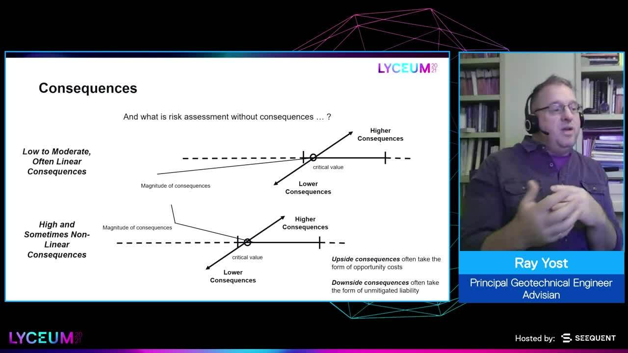
And the other half of risk is the of course, consequences.

[00:09:51.810]
And our consequences can like sensitivity

[00:09:54.450]
be low to moderate.

[00:09:56.460]
As we’re changing that input value,

[00:10:00.020]
we don’t really see a change in the consequence that much.

[00:10:04.210]
So say again factor of safety in a stability analysis

[00:10:07.850]
is our example.

[00:10:12.200]
And we’re reducing that input material strength,

[00:10:15.440]
and we’re getting a failure.

[00:10:16.780]
But the size of the failure

[00:10:18.090]
is not really changing,

[00:10:19.670]
the run-out distance isn’t changing.

[00:10:21.780]
We’re not really seeing huge differences

[00:10:24.640]
in the consequences of that,

[00:10:26.900]
even though the factor of safety might be dropping,

[00:10:28.780]
it’s not really having an effect

[00:10:30.290]
on what the impacts of that would be.

[00:10:33.213]
So we can have this lower,

[00:10:35.330]
and again, linear consequences

[00:10:37.500]
as we go down this potential range of uncertainty,

[00:10:42.396]
or we can have very high consequences,

[00:10:44.620]
and even non-linear consequences again.

[00:10:48.060]
Now one note on the consequences,

[00:10:50.150]
we have both downside consequences.

[00:10:53.230]
These are often going to take

[00:10:54.230]
the form of unmitigated liability.

[00:10:56.560]
And why I say liability instead of risk,

[00:10:58.740]
is that it’s sort of the next piece.

[00:11:02.740]
Things could be worse than we assume,

[00:11:05.410]
higher risks, and then these risks

[00:11:07.330]
haven’t been attenuated or mitigated

[00:11:09.040]
because we aren’t aware of them,

[00:11:11.610]
and that’s going to create a liability.

[00:11:13.290]
So that’s the downside consequences,

[00:11:15.490]
this unmitigated liability.

[00:11:17.830]
And the upside consequences are going to be more

[00:11:19.950]
in the form of opportunity costs.

[00:11:22.630]
Essentially we could have had a leaner, meaner construction

[00:11:27.490]
of whatever sort.

[00:11:28.323]
We didn’t have to have a to have slope angle that was that shallow.

[00:11:32.660]
We didn’t have to have an embankment that was that big.

[00:11:35.290]
We dedicated resources to something

[00:11:37.030]
that we didn’t need to necessarily

[00:11:38.880]
to achieve our desired outcome in terms of safety.

[00:11:42.900]
Next slide, please.

[00:11:47.000]
So given this construct with sensitivity,

[00:11:50.230]
greater or lesser than,

[00:11:52.210]
the asymmetry in the outcome upside or downside,

[00:11:57.370]
and then the consequences either higher or lower.

[00:12:00.310]
We have this box of possibilities

[00:12:02.040]
in terms of these risks scenarios now,

[00:12:04.410]
and uncertainty scenarios

[00:12:06.790]
that we’ve got eight different circumstances

[00:12:09.510]
that we can look at

[00:12:11.020]
in terms of all of these different ways

[00:12:12.760]
we can think about risk as a function of uncertainty.

[00:12:17.530]
Next slide, please.

[00:12:22.180]
So we’ve talked about now

[00:12:23.655]
the first two pieces of that flow diagram

[00:12:28.070]
that I showed in the earlier slide

[00:12:30.220]
with uncertainty and assumptions.

[00:12:32.630]
That’s how we start to think about risk.

[00:12:34.740]
Now we talk about the analysis and the risk mitigation,

[00:12:37.670]
and this is through the tools that we use.

[00:12:40.521]
These are all these different tools

[00:12:42.250]
that are available to us as geotechnical engineers

[00:12:44.670]
to address this uncertainty.

[00:12:47.050]
How do we think about uncertainty?

[00:12:50.980]
I won’t say that this is the definitive way

[00:12:53.280]
to think about these tools,

[00:12:55.620]
but I will say that there is a continuum of sorts

[00:12:58.410]
between all these different tools that we have.

[00:13:00.390]
And this slide isn’t meant to capture all the tools

[00:13:02.830]
that are available to us as geotechnical engineers.

[00:13:05.670]
But to talk about them in terms of these broad categories,

[00:13:10.310]
where we have tools

[00:13:11.520]
that are based in inductive reasoning and inference,

[00:13:15.600]
these are things like the first picture

[00:13:17.980]
where we have something about A that we don’t know.

[00:13:21.110]
This could be again, a material strength.

[00:13:23.850]
We know a lot about A, or something about A,

[00:13:27.880]
we tend to know a lot more about B

[00:13:29.670]
including that material strength

[00:13:31.070]
this target thing we want to know.

[00:13:32.510]
And A and B share enough characteristics

[00:13:35.630]
that we can assume that whatever material strength B has,

[00:13:38.560]
A has the same strength or similar strength.

[00:13:42.320]
We have tools that fall into this

[00:13:43.730]
sort of proportional relationship.

[00:13:46.036]
A is somehow relative to B,

[00:13:48.180]
think about, we have a few compressive strength samples

[00:13:51.810]
where we’ve incurred the higher cost

[00:13:53.060]
to do the compressive strength testing

[00:13:55.380]
and a whole lot of point load samples.

[00:13:58.250]
And there’s a proportionality between those two.

[00:14:00.270]
So we can look at the range

[00:14:02.250]
of compressive strength variation

[00:14:05.800]
as a function of the range of point load strength variation.

[00:14:11.160]
There’s a lot more, of course,

[00:14:12.320]
again, these are not meant to be exhaustive lists

[00:14:15.350]
of all these different tools,

[00:14:16.440]
just to get the sense of what an inference

[00:14:20.220]
or inductive reasoning type of tool looks like.

[00:14:23.720]
We have parametric tools, or these are basically

[00:14:26.880]
this one of the kitchen-sink approach.

[00:14:29.310]
We’re throwing a lot of different things

[00:14:31.460]
in sampling from them into a bin.

[00:14:34.840]
This can be a lot of different types of variables.

[00:14:37.330]
And we’re trying to come up

[00:14:38.470]
with some sort of parametric analysis

[00:14:40.980]
based on Monte Carlo, Latin Hypercube sampling, whatever

[00:14:44.560]
that produces this range of outcomes.

[00:14:46.900]
And we can start to look at that range of outcomes

[00:14:48.970]
and make some conclusion from that.

[00:14:52.730]
There’s a lot of things around say subjective probability

[00:14:55.810]
that might fall into this as well.

[00:14:59.220]
A lot of different tools

[00:15:00.240]
where we’re basically just looking at

[00:15:02.640]
what the distributions are

[00:15:04.170]
across a lot of different ranges of our variables.

[00:15:08.050]
And then we have these direct

[00:15:09.130]
or deductive reasoning types of tools

[00:15:11.977]
where we’re just either looking at

[00:15:14.340]
what information we have, this is the variation,

[00:15:17.180]
or maybe we’re extrapolating from something.

[00:15:19.460]
A lot of times frequency or recurrence interval

[00:15:23.320]
might fall into these types of deductive reasoning tools.

[00:15:27.220]
We have a bunch of data from a time history,

[00:15:29.455]
and we’re going to extrapolate that out a little bit

[00:15:31.867]
and pretty much this is what we can assume

[00:15:33.930]
about the circumstance from the information we have.

[00:15:37.780]
We could also assume some cases, just the minimum value.

[00:15:40.790]
If we know that the range is bound in a certain way,

[00:15:45.940]
it starts at zero, it goes to a hundred,

[00:15:48.120]
maybe we pick one or the other

[00:15:49.340]
as far as an upper or lower bound to what that would be.

[00:15:53.590]
So these things as well,

[00:15:54.730]
I’m going to argue, fall on a continuum.

[00:15:56.850]
There’s not any necessarily hard lines between them but–

[00:16:01.940]
Next slide, please.

[00:16:02.990]
We will talk about the relative strengths

[00:16:06.140]
and weaknesses of them.

[00:16:07.510]
And again, not meant to be an exhaustive list

[00:16:09.780]
just to illustrate that each of these has a place and a use

[00:16:14.480]
in terms of addressing uncertainty.

[00:16:17.250]
With inference and inductive reasoning,

[00:16:20.370]
a lot of times we’re using a lot of our knowledge

[00:16:23.610]
and understanding as geotechnical engineers

[00:16:25.590]
to relate one thing to another,

[00:16:27.940]
or use some other bit of data to modify

[00:16:33.330]
or increase the precision of our estimate.

[00:16:35.342]
We could say, if we don’t know a material strength,

[00:16:39.250]
we can assume it’s zero, that’s pretty conservative.

[00:16:42.140]
We don’t want to do that necessarily,

[00:16:43.990]
so we’re using inference

[00:16:46.140]
to increase the precision of that estimate.

[00:16:49.370]
Of course, the weakness of this,

[00:16:50.620]
it it’s really based on knowledge

[00:16:52.380]
from practitioner to practitioner, that can vary.

[00:16:55.340]
I might be really good at estimating material strength

[00:16:57.970]
from all these other materials strengths that I’m aware of,

[00:17:00.640]
the next person has maybe more of a limited expertise

[00:17:05.340]
in that area.

[00:17:06.670]
And you’re going to get very different answers

[00:17:08.190]
from inference and inductive reasoning

[00:17:10.280]
from practitioner to practitioner,

[00:17:12.110]
probably the basis of a lot of arguments

[00:17:13.780]
that we have as geological engineers.

[00:17:18.450]
The direct or deductive reasoning,

[00:17:20.760]
the strength there is that

[00:17:22.230]
since you’re assuming either from what you know,

[00:17:26.250]
or from more importantly from some end value of this,

[00:17:33.420]
you sort of covered all the bases.

[00:17:35.330]
You’re not going to be surprised

[00:17:37.140]
by something that wasn’t captured in your assumption.

[00:17:40.130]
The weakness of course,

[00:17:41.040]
is that these can be fairly conservative estimates.

[00:17:44.730]
With the parametric tools,

[00:17:48.030]
the strength is that it’s actually

[00:17:50.260]
kind of drawing on the strengths

[00:17:51.640]
of both inference and inductive reasoning

[00:17:54.640]
as well as direct and deductive reasoning.

[00:17:57.440]
And so it’s pulling the best of each of those.

[00:18:00.770]
The weakness is that

[00:18:02.230]
this can require considerable time expertise.

[00:18:04.942]
You would have to pull from a lot of different people.

[00:18:07.880]
You’re going to have to deal

[00:18:08.860]
with some of those issues around,

[00:18:10.450]
again, both of the weaknesses of each method.

[00:18:13.760]
The other one that it can cause

[00:18:16.490]
is that you end up with this range of possible outcomes

[00:18:20.180]
that’s going to vary

[00:18:21.900]
from some extreme adverse outcome to extreme good outcome,

[00:18:27.224]
and you’re going to have to make some decisions

[00:18:29.780]
around which one’s going to be the appropriate outcome.

[00:18:32.610]
How do you decide?

[00:18:33.500]
Do you have a cluster of outcomes around a central value?

[00:18:37.490]
And that’s a good thing.

[00:18:38.720]
Or do you have these long tails

[00:18:40.790]
that you have to make some decisions about?

[00:18:43.590]
It can sort of solve some of the problems

[00:18:46.127]
of inference or deductive reasoning on the front end,

[00:18:50.300]
but cause more problems on the backend.

[00:18:53.230]
So no one tool is perfect,

[00:18:55.990]
but they all have their advantages and disadvantages.

[00:18:59.460]
So next slide.

[00:19:02.580]
So now we’ve compartmentalized

[00:19:05.200]
all these different circumstances of uncertainty and risk,

[00:19:10.340]
and now we have the different tools that we apply.

[00:19:12.930]
And we’re going to start talking about

[00:19:15.100]
how each of those tools fits

[00:19:17.030]
each of these different circumstances.

[00:19:19.030]
So we have that box of possibilities

[00:19:21.270]
from the previous slide,

[00:19:22.190]
and we split it,

[00:19:23.340]
and we’re looking at the downside on the left side,

[00:19:26.140]
and the upside on the right side.

[00:19:28.130]
We can start to look at how these tools

[00:19:30.330]
apply to these different circumstances

[00:19:33.140]
as a function of sensitivity and consequence,

[00:19:36.490]
and then upside or downside risk.

[00:19:39.310]
So I’d like to talk about these for a little bit,

[00:19:41.950]
and I’ll start with the downside risk

[00:19:44.160]
in the lower left-hand corner.

[00:19:47.070]
We have a situation where we have pretty low consequences,

[00:19:50.350]
pretty low sensitivity, or in sensitivity,

[00:19:53.720]
it’s downside risk, but essentially you’re not going to,

[00:19:57.380]
because of this insensitivity and lower consequences,

[00:20:02.360]
you can assume fairly extreme values

[00:20:05.530]
without really any cost in terms of allocation of resources.

[00:20:09.220]
So that’s a pretty good place for that tool to sit.

[00:20:12.650]
In this middle band,

[00:20:14.087]
we have either the higher consequences

[00:20:17.043]
with the higher sensitivity,

[00:20:19.105]
(coughing) excuse me.

[00:20:20.765]
Some of these inductive tools are going to be more important

[00:20:24.680]
because now either we have to think about consequences

[00:20:29.690]
or we have to think about that sensitivity.

[00:20:31.330]
We do want a little bit more precision

[00:20:33.394]
in how we approach this.

[00:20:34.890]
We want to be aware of implausible or extreme values

[00:20:40.320]
and how those might affect our answer,

[00:20:42.065]
but we don’t want to let them influence our answer too much

[00:20:46.490]
because they could lead to such an extreme outcome

[00:20:49.250]
in our risk assessment

[00:20:50.410]
that we’re, again, misallocating resources.

[00:20:52.610]
So we want to start using some of these inference tools

[00:20:55.140]
to increase the precision of our input assumptions.

[00:20:59.400]
And then finally, when we get to the upper right side

[00:21:02.180]
on the upper right quadrant on the downside risk,

[00:21:06.698]
it really speaks to,

[00:21:08.150]
we have a lot of sensitivity, high consequences.

[00:21:10.870]
We need to look at this parametric approach

[00:21:12.700]
because we want to capture potentially some relationships

[00:21:15.970]
between different, either within a variable

[00:21:19.410]
or due to non-linear responses,

[00:21:22.330]
or maybe some combination of variables

[00:21:24.315]
that may not be intuitive.

[00:21:26.720]
We really want to see what that full range of outcomes

[00:21:29.180]
looks like.

[00:21:30.770]
So for the upside,

[00:21:33.780]
we have a similar set of different tools

[00:21:36.433]
that are going to be applied to these different compartments,

[00:21:40.340]
but a slight difference.

[00:21:41.602]
If we start in the lower right-hand corner of this time,

[00:21:46.490]
we have low sensitivity, low consequences,

[00:21:49.060]
but because it’s more of a matter of opportunity costs,

[00:21:52.790]
we want to use this parametric approach

[00:21:54.830]
to understand those a little bit better.

[00:21:58.450]
There’s some value in looking at those

[00:22:00.850]
so that we’re understanding

[00:22:01.870]
that we’re again, allocating resources appropriately.

[00:22:05.380]
For these middle two boxes

[00:22:07.263]
where we have the higher consequences, but less sensitivity,

[00:22:11.730]
these again, these indirect and inductive reasoning methods

[00:22:14.950]
are important to increase that precision around our answer.

[00:22:20.800]
But once we get into the lower consequences

[00:22:23.620]
with greater sensitivity,

[00:22:25.360]
the direct and deductive approaches

[00:22:27.320]
are more important to use.

[00:22:30.040]
And of course, when we get up

[00:22:31.130]
into the upper left quadrant there

[00:22:34.370]
with greater sensitivity and higher consequences,

[00:22:37.760]
we want to use those parametric approaches

[00:22:39.616]
again, to understand

[00:22:41.520]
if there’s some sort of non-intuitive outcome

[00:22:44.810]
that we can experience,

[00:22:46.795]
or to look at whether those outcomes are clustered

[00:22:50.400]
around some sort of central value

[00:22:52.100]
or have these longer tails

[00:22:53.610]
that might be important to consider.

[00:22:55.650]
Again, it speaks to

[00:22:57.600]
how do we start to look at the tools

[00:23:00.410]
versus the circumstance

[00:23:01.561]
to properly mitigate risk

[00:23:05.930]
or allocate resources to mitigate risk.

[00:23:08.730]
Next slide, please.

[00:23:12.510]
So where do we come to with all this?

[00:23:15.450]
We can use this relationship between what we do know

[00:23:19.590]
and the range of what we may not know or don’t know

[00:23:23.156]
to think about how to characterize uncertainty

[00:23:26.930]
relative to risk.

[00:23:29.520]
And you can agree or disagree

[00:23:31.330]
with any parts of this discussion

[00:23:34.810]
or any parts of my presentation.

[00:23:38.160]
What it does come down to

[00:23:39.410]
again, is this fundamental idea

[00:23:42.290]
that we can discuss this and go on and on

[00:23:45.540]
and talk about our different approaches and whatnot.

[00:23:50.460]
But we do have to think at the end of the day

[00:23:52.340]
about that allocation of resources.

[00:23:54.800]
And so the purpose of all this

[00:23:56.540]
is just to highlight

[00:23:57.730]
that there is this structure to uncertainty.

[00:24:01.081]
There are impacts that the tools

[00:24:03.940]
that we use as geological engineers have

[00:24:06.160]
to how we think about that.

[00:24:07.750]
And when we start to marry those two

[00:24:10.230]
and look at the circumstances of uncertainty

[00:24:13.140]
and the tools that we have for addressing it,

[00:24:16.790]
we really want to make sure that that’s a good marriage

[00:24:19.900]
in terms of producing this optimal allocation of resources

[00:24:24.970]
at the end of the day.

[00:24:26.520]
And that’s really the message of this entire talk.

[00:24:31.260]
Next slide, please.

[00:24:33.870]
Thank you for your time and attention.

[00:24:35.258]
(upbeat music)