В этом видеоролике рассказывается о динамической связи между Leapfrog Geo и ioGAS и о том, как можно использовать надежные рабочие процессы для максимально эффективного использования геохимических и литологических данных.

В данном видеоролике рассматриваются:

Отправка данных интервалов и точечных данных Leapfrog Geo в ioGAS
Анализ данных и назначение атрибутов в ioGAS
Усовершенствованные процессы для работы с данными геохимии
Визуализация геохимических данных в трехмерном Рабочем окне Leapfrog Geo по прямому каналу связи
Импорт данных из ioGAS в виде точек или интервалов
Построение геологических моделей и интерполянтов на основе геохимических данных

Обзор

спикеров

Путра Садикин (Putra Sadikin)
Старший аналитик программного обеспечения — Imdex Limited

Аллан Игнашио (Allan Ignacio)
Старший геолог проекта — Seequent

Продолжительность

1 час 6 минут

Смотреть больше видео по запросу

Видео

Узнайте больше о решении Seequent для горнодобывающей промышленности

Узнать больше

Расшифровка видеозаписи

<!— wpml:html_fragment —>
[00:00:00.065] (gentle music)
[00:00:06.440] <encoded_tag_open />v Allan<encoded_tag_closed />I am Allan Ignacio senior project geologist here<encoded_tag_open />/v<encoded_tag_closed />
[00:00:09.140] at Seequent based in Perth,
[00:00:11.270] and I’ve over 25 years experience
[00:00:13.470] with the exploration and resource evaluation.
[00:00:16.640] My co-presenter is Putra Sadikin,
[00:00:19.760] an experienced geochemist and senior software analyst
[00:00:22.510] from Imdex Limited.
[00:00:24.130] Putra, can you tell more about yourself?
[00:00:26.650] <encoded_tag_open />v Putra<encoded_tag_closed />Thanks, Allan.<encoded_tag_open />/v<encoded_tag_closed />
[00:00:28.010] It’s a pleasure to be here to be presenting this webinar
[00:00:31.140] with you guys today.
[00:00:32.440] So I work in a product management team
[00:00:34.650] for the ioGAS software.
[00:00:36.500] I look after product support training,
[00:00:38.760] and a bit of sales and research
[00:00:40.430] and development work for the software.
[00:00:42.970] My background is in geology.
[00:00:44.790] Today, we’ll be presenting a bit of a workflow
[00:00:48.140] between ioGAS and Leapfrog Geo and I’m really excited
[00:00:50.940] to be here today.
[00:00:52.080] Thanks Allen.
[00:00:53.530] <encoded_tag_open />v Allan<encoded_tag_closed />Thank you Putra.<encoded_tag_open />/v<encoded_tag_closed />
[00:00:54.890] So today’s presentation is about linking lithology
[00:00:58.340] and Geochemistry through the use of Leapfrog Geo and ioGAS.
[00:01:02.670] The purpose of this presentation
[00:01:04.250] is for us to appreciate the live link
[00:01:05.910] between Leapfrog Geo and ioGAS,
[00:01:08.780] as well as have the opportunity
[00:01:10.180] to analyze various multi element data,
[00:01:13.360] which could provide hints
[00:01:14.530] to determine different rock types, alteration,
[00:01:17.470] and mineralization patterns
[00:01:19.320] that normally our naked eye couldn’t immediately see.
[00:01:23.420] So for today’s webinar,
[00:01:24.910] we’ll first give you an overview about our company,
[00:01:27.606] then I’ll be going through a series of PowerPoint slides
[00:01:30.670] on sequence solutions, including Leapfrog Geo
[00:01:34.820] and ioGAS link, we’ll give you a bit
[00:01:37.030] of background about the dataset that we used
[00:01:39.490] for multi-element analysis
[00:01:41.640] before moving into the Leapfrog Geo
[00:01:44.665] and ioGAS workflows, which I’m pretty sure all
[00:01:46.920] of you will find interesting and useful.
[00:01:49.045] And then we’ll jump into the live demo
[00:01:51.620] on Leapfrog Geo and ioGAS workflows,
[00:01:54.580] and then end it with a summary.
[00:01:58.070] So about Seequent.
[00:01:59.070] Seequent is a global leader
[00:02:01.420] in the development of visual data science software
[00:02:05.670] and collaborative technologies.
[00:02:08.310] We turn complex data into geological understanding,
[00:02:11.770] provide timely insights,
[00:02:13.437] and gave decision-makers confidence that they need.
[00:02:17.480] Our Seequent solutions harness information,
[00:02:20.460] extract value, bring meaning, and reduce risk.
[00:02:25.200] Our 3D modeling tools
[00:02:26.550] and technology are widely applied across industries
[00:02:30.755] and projects, including road and tunnel construction,
[00:02:34.620] groundwater detection and management,
[00:02:37.540] geothermal exploration, we also have something
[00:02:41.247] in resource evaluation and estimation, subterranean storage
[00:02:47.220] of spent nuclear fuel and a whole lot more.
[00:02:50.410] So the sequence solution encompasses a range
[00:02:52.670] of software products applicable for use
[00:02:55.740] across the volume mining chain.
[00:02:59.100] We have the Geosoft suite of products
[00:03:02.480] and the Leapfrog suite of products, both for GIS mapping,
[00:03:07.040] geophysical, geochemical, geological, and resource modeling,
[00:03:12.450] and we also have the GEOSLOPE products
[00:03:14.630] that are designed for geotechnical engineering problems.
[00:03:18.930] I’m sure many of you are already familiar
[00:03:20.770] with some of these solutions.
[00:03:23.000] Most can be integrated using Seequent Central
[00:03:26.220] for model management and collaboration.
[00:03:29.780] Today, we will be focusing on Leapfrog Geo, ioGAS,
[00:03:33.940] and index product, and the Leapfrog Geo-ioGAS link
[00:03:37.790] so that we can visualize geochemical data in real-time.
[00:03:42.550] So what is Leapfrog Geo?
[00:03:45.257] Leapfrog Geo is workflow based 3D
[00:03:48.220] implicit geological modeling tool,
[00:03:50.680] which allows you to quickly construct models
[00:03:53.480] directly from various sources,
[00:03:56.110] including drill holes, points, and surfaces.
[00:04:00.640] Leapfrog uses volumetric algorithm called Fast RBF
[00:04:05.230] to construct fast pass surfaces quickly.
[00:04:08.520] The RBF or radial basis function
[00:04:11.510] is a mathematical backbone of Leapfrog.
[00:04:14.490] The surfaces such as in here in the 3D scene.
[00:04:18.820] Created, can be modified as needed
[00:04:21.130] to fit your geological interpretations.
[00:04:24.280] So due to its implicit nature,
[00:04:26.680] your models can be dynamically updated
[00:04:28.810] to honor new input data at any time.
[00:04:32.490] This new data can be new drilling information,
[00:04:35.650] new surface information, or any useful inputs.
[00:04:40.240] Under the geochemistry folder is the ioGAS link.
[00:04:44.680] We’re going to use this tool to bring assay data
[00:04:47.690] from Leapfrog Geo as points or interval file
[00:04:51.300] to ioGAS, where you can interrogate, visualize,
[00:04:57.103] and classify data, then back to Leapfrog Geo,
[00:05:00.030] where you can visualize and model the data.
[00:05:04.370] I’m now handing over to Putra,
[00:05:06.290] who will explain more about ioGAS, Putra?
[00:05:10.950] <encoded_tag_open />v Putra<encoded_tag_closed />Thank you, Allan, and thanks for the introduction.<encoded_tag_open />/v<encoded_tag_closed />
[00:05:13.690] So for those of you who have not heard
[00:05:16.170] or used ioGAS software before,
[00:05:18.640] I just want to give a brief introduction
[00:05:21.333] of what ioGAS is and why we do what we do here.
[00:05:25.130] So ioGAS is developed by Imdex, a mining tech company,
[00:05:29.210] specializing in development of cloud connected devices
[00:05:33.790] and drilling optimization products
[00:05:35.540] to improve the process of identifying
[00:05:38.360] and extracting mineral for resource companies.
[00:05:41.040] And as a program,
[00:05:42.270] ioGAS has been around for more than 10 years now.
[00:05:45.440] It’s a software that lets you
[00:05:47.160] interpret your geoscientific data.
[00:05:50.040] We have years of experience supplying high-level advanced
[00:05:53.170] data analysis techniques to your practical applications
[00:05:56.670] in interpreting your geochemical and other geological data
[00:06:00.860] such as downhole gamma measurements and structural logging.
[00:06:04.980] So what we do best in ioGAS
[00:06:06.900] is in applying exploratory data analysis techniques
[00:06:10.830] to your geochemical data.
[00:06:12.560] And that is our focus through our very visual workflow.
[00:06:16.980] And that workflow in itself is suitable
[00:06:19.360] for looking at our data types as well.
[00:06:21.370] So it’s not just for your geochemistry data,
[00:06:24.410] so you can use the workload that we have
[00:06:26.340] in the program to interrogate spectral data
[00:06:29.110] such as those from Osiris and structural data,
[00:06:32.020] such as the ones that we get from our Iq other tool,
[00:06:34.980] also our downhole gamma data
[00:06:36.960] from our easy gamma tool as well.
[00:06:39.330] So that’s ioGAS.
[00:06:41.790] So this is an example
[00:06:43.210] of a typical workflow window for ioGAS.
[00:06:47.050] So this is an example of someone who wants to know more
[00:06:50.120] about the geological context behind his geochemical data.
[00:06:55.140] So say, if you got your assay data
[00:06:57.630] from the lab that corresponds to a draft that you upload
[00:07:01.590] from the field, and you just want to know more
[00:07:04.075] about them, about the context, about their background,
[00:07:09.430] and what processes can be inferred from this.
[00:07:12.090] So you can see on the right-hand side
[00:07:14.050] of this window is a couple of classification diagrams.
[00:07:17.730] So this is what we call X, Y
[00:07:20.480] or ternary scatterplots with overlays of shape and lines.
[00:07:24.340] So polygons and polylines
[00:07:26.340] that allows someone to classify their data points.
[00:07:30.410] And it’s a way for geologists
[00:07:33.230] to link back their geochem data
[00:07:36.200] to certain geological classification
[00:07:39.450] based on known composition
[00:07:41.470] and also infer certain geological processes.
[00:07:45.530] So it’s a process reduction technique.
[00:07:48.750] So it’s a way for someone
[00:07:50.000] to visualize their geochemical data
[00:07:53.881] in the 2D or 3D space
[00:07:56.865] and allowing them to link it back to what they know
[00:07:59.010] about the rocks, either from visual logging
[00:08:03.145] or from other ways that they have interpreted their data.
[00:08:06.000] And next to it in the middle, we have our decision tree.
[00:08:09.420] So that’s what we call our classification
[00:08:11.650] and regression tree algorithm.
[00:08:14.030] So this is a way for someone
[00:08:15.550] to figure out which elements contribute the most
[00:08:18.380] to classifying the data points based on
[00:08:21.374] their geology and what they have locked
[00:08:23.930] in the field and things like that.
[00:08:25.720] And next to it, just on the left is a wavelet plot.
[00:08:30.260] And that is a way for someone to define their boundaries
[00:08:35.448] using downhole data from either their instrumentation
[00:08:39.900] from gamma data or their geochemistry data
[00:08:43.800] that they plotted up on a downhole plot, such as this one.
[00:08:46.180] So it’s allowing them to automatically pick up boundaries
[00:08:49.264] and enabling them to make better decisions
[00:08:53.280] on where your boundaries are sitting
[00:08:55.290] with respect to alteration or lithological processes.
[00:08:58.890] And just on the very left
[00:08:59.980] is a couple of principal components analysis plots.
[00:09:04.160] So in the bottom is an example of a biplot.
[00:09:07.020] So you’re plotting up in the result
[00:09:09.280] of principal components analysis on your data points,
[00:09:13.360] and you’re plotting up the principal components access
[00:09:16.130] on top of it.
[00:09:17.180] And you’re just basically seeing which elements contribute
[00:09:19.590] the most to the variation that’s represented
[00:09:22.990] by the data points.
[00:09:23.990] And you’re linking, basically linking all these processes
[00:09:27.710] that you’re able to identify using classification diagrams
[00:09:31.470] and with some mathematical analysis as well to back that up.
[00:09:35.620] So we will go through some
[00:09:37.800] of these in more detail, especially on the right-hand side
[00:09:40.600] of the screen with the classification diagrams.
[00:09:43.180] We’ll go through this workflow
[00:09:44.340] in more detail within this webinar.
[00:09:46.300] So thanks, Allan.
[00:09:49.040] <encoded_tag_open />v Putra<encoded_tag_closed />Thank you Putra for a brief introduction on ioGAS.<encoded_tag_open />/v<encoded_tag_closed />
[00:09:53.750] I’m now going to show you some information
[00:09:55.920] about the dataset that we’re going to use.
[00:09:58.780] So there are 11 drill holes in this project.
[00:10:02.320] So displayed on the 3D scene are the different rock types.
[00:10:05.730] We’ve got two felsic rocks, A and B,
[00:10:08.465] and we’ve got a mafic rock,
[00:10:11.230] which is the dark blue in color.
[00:10:13.700] We have a total of 1084 data points
[00:10:18.228] with 59 assays per suite per interval.
[00:10:22.620] Displayed on the right side of the screen are tables
[00:10:25.160] for your color for assay, and also for your geology.
[00:10:30.730] Assay data is composed
[00:10:32.060] of major, immobile, rare earth elements,
[00:10:35.910] precious and base metals.
[00:10:37.750] This assay groups can be viewed in ioGAS.
[00:10:41.190] Once again, and I’ll hand over to Putra
[00:10:42.940] who’ll briefly discuss the Leapfrog Geo and ioGAS workflows.
[00:10:47.750] Off to you, Putra.
[00:10:50.090] <encoded_tag_open />v Putra<encoded_tag_closed />Thanks, Allan.<encoded_tag_open />/v<encoded_tag_closed />
[00:10:51.150] So just jumping off on this slide a bit.
[00:10:53.850] So this is a display
[00:10:55.040] of how you would select your elements in ioGAS.
[00:10:58.810] And what we provide to our users
[00:11:00.880] is a way of easily selecting
[00:11:03.970] from a list of provided elements based on common groupings.
[00:11:09.900] So major elements, immobiles, and rare elements,
[00:11:13.225] they’re grouped in a certain way
[00:11:15.933] that we can pick them easily from ioGAS
[00:11:18.660] and they also provide a list of pathfinder elements
[00:11:21.480] for common deposit types and that sort of thing.
[00:11:24.000] So this is just a way for you to group your elements
[00:11:27.070] together before you visualize them within ioGAS.
[00:11:31.630] So I’m just going to go through the workflow
[00:11:34.770] that we’re going to be presenting to you today.
[00:11:37.700] So the first workflow is igneous rock classification.
[00:11:41.690] So this is what we will do
[00:11:44.320] to look at your geochem data in ioGAS.
[00:11:50.150] So we’re going to bring intervals data containing assay
[00:11:54.540] information from Leapfrog Geo into ioGAS.
[00:11:58.260] And we are going to use a combination
[00:12:01.810] of classification diagrams
[00:12:04.120] in ioGAS to classify the rocks based on certain processes
[00:12:08.520] and what we think are actually happening behind the data
[00:12:14.430] on its own.
[00:12:15.360] And what we ended up actually discovering from this
[00:12:18.320] is we were able to subdivide our log classification.
[00:12:23.280] So not just felsic A, felsic B, and mafic
[00:12:25.930] we were able to actually split them up into sub groups,
[00:12:29.270] just using a combination of relatively simple
[00:12:32.900] geochemical classification diagrams.
[00:12:35.180] And what we’re able to do in ioGAS
[00:12:36.970] is we’re able to save them as a new column,
[00:12:42.960] and we’re able to push that across back to Leapfrog Geo,
[00:12:46.170] where Allan is able to turn them into
[00:12:50.170] a refined geological model
[00:12:52.940] based on our geochemical classification.
[00:12:55.730] That’s what we call the back flagging process.
[00:12:58.530] And moving on to the second workflow.
[00:13:01.620] So we were able to take this one step further
[00:13:05.090] and we will again use a combination
[00:13:07.210] of simple classification diagrams,
[00:13:09.840] and in this case, a combination of the alteration box plot,
[00:13:13.400] and a couple of molar element ratio diagrams
[00:13:17.986] to identify the processes really
[00:13:21.980] that we can observe here in this rock.
[00:13:23.710] So it’s important for us to
[00:13:26.860] go through the process of first identifying
[00:13:29.450] the lithology before we delve into the alteration.
[00:13:32.850] But the way that we’ve used this alteration modeling
[00:13:36.020] is we were able to identify the data points
[00:13:39.410] that corresponds to the processes that we were able
[00:13:41.930] to see using these diagrams.
[00:13:43.990] And then through the creation of new color groups,
[00:13:47.410] based on this information, that’s in a new column
[00:13:50.490] in ioGAS that we are able to backtrack into the Leapfrog Geo
[00:13:55.020] as a way for someone like Allan
[00:13:57.420] to create the new alteration model
[00:14:00.320] based on the alteration modeling
[00:14:02.290] that we’ve come up within ioGAS.
[00:14:05.290] So that’s the essence of today’s webinar.
[00:14:08.160] And I’ll hand over the control
[00:14:09.520] to Allan who will go through the process,
[00:14:11.700] starting from the Leapfrog Geo side of it.
[00:14:13.680] Thanks, Allan.
[00:14:15.518] <encoded_tag_open />v Allan<encoded_tag_closed />Thank you, Putra.<encoded_tag_open />/v<encoded_tag_closed />
[00:14:17.180] So let’s now jump into the live demo
[00:14:19.200] on Leapfrog Geo and ioGAS.
[00:14:21.670] Have now opened Leapfrog Geo together
[00:14:24.260] with a lithological model that we have previously created,
[00:14:28.500] it’s a very simple model.
[00:14:30.370] It contains three lithologies, felsic A, felsic B,
[00:14:34.190] and the mafic rock.
[00:14:36.380] Again, for those who are not too familiar with Leapfrog,
[00:14:39.850] just as a brief rundown on the user interface
[00:14:43.080] we have in here, the project tree on the left side
[00:14:47.400] of the screen, which is designed with a top-down approach.
[00:14:51.600] The first half of the folders,
[00:14:53.300] so from topography down to around like meshes folder.
[00:14:58.560] So this is where data is imported or created.
[00:15:02.210] And the second half is where all the various models
[00:15:05.100] are going to be constructed.
[00:15:06.710] So from the geological models folder
[00:15:09.790] down to the block models folder.
[00:15:12.490] And of course, you’ve got in here to save scenes and movies,
[00:15:16.620] sections and contours for presentation purposes,
[00:15:20.960] and lastly, we have in here a folder
[00:15:23.520] for a geochemical analysis, of course.
[00:15:25.550] And you also have in here
[00:15:27.000] an option to import color gradients.
[00:15:30.680] We also have in here the 3D scene
[00:15:32.480] in the middle where you can interact objects,
[00:15:35.080] where as you can drag and drop things from the project tree
[00:15:39.280] to the 3D scene and everything
[00:15:41.840] that is displayed on the 3D scene is actually listed down
[00:15:46.010] in here under the shape place at the bottom of the 3D scene.
[00:15:50.770] We can choose the different visualization settings
[00:15:53.650] such as turning on and off layers,
[00:15:57.740] turning on and off objects,
[00:16:01.010] or determining what you want to visualize in the 3D scene.
[00:16:06.640] So underneath the save scenes folder,
[00:16:08.760] I’m just going to expand this particular folder over here.
[00:16:12.300] I’ve created a few save scenes, which act as bookmarks.
[00:16:16.710] I’ll be running through this
[00:16:17.860] for the purposes of this presentation.
[00:16:21.170] This is a great way of preserving perspectives
[00:16:23.640] of different objects or to tell a story
[00:16:25.631] without bringing different objects into the scene.
[00:16:29.840] So one of the more important features mentioned earlier
[00:16:33.180] is that Leapfrog Geo is dynamic in nature.
[00:16:36.840] So any changes that you make
[00:16:38.880] to the data will automatically be reflected throughout.
[00:16:43.480] So I’m just going to go through
[00:16:44.490] with the following save scenes now.
[00:16:48.250] So these are the colors of the drill holes,
[00:16:52.570] and I’m going to just going to display the assay now
[00:16:55.060] with scandium and also titanium.
[00:17:00.230] So I’ve just set in here two examples
[00:17:01.533] by displaying scandium and titanium.
[00:17:04.330] However, under the drop down in here under the assay table,
[00:17:07.890] feel free to, you can choose whatever elements you want
[00:17:11.410] to display, for example, nickel.
[00:17:15.720] Just going to go through with the geology again.
[00:17:19.320] So these are displaying the three major deformities,
[00:17:23.370] felsic A, felsic B, and the mafic rock.
[00:17:26.880] The first thing that we’re going to do
[00:17:28.530] is we’re going to construct a surface
[00:17:30.420] in between felsic A and B.
[00:17:33.990] So I’ve created an intrusion surface in here
[00:17:37.255] to model between the two lithologies.
[00:17:41.300] And after that, I was able to model the mafic rock
[00:17:45.280] as a vein.
[00:17:47.680] And then from there,
[00:17:49.173] I was able to create the simple lithogical model.
[00:17:52.500] So everything happens under the geological models folder.
[00:17:56.120] I’m just going to expand this a bit more
[00:17:58.310] and all the surfaces
[00:17:59.650] are created under the surface chronology
[00:18:01.940] by right clicking on it.
[00:18:03.860] And then by creating the output volumes of course,
[00:18:05.785] for those who of familiar,
[00:18:07.910] just double click on the surface cohomology
[00:18:10.170] we activate the surfaces, click okay,
[00:18:12.980] and we create the output volumes down in here.
[00:18:17.910] Okay, let’s move on.
[00:18:18.777] And I’m just going to kind of slice through
[00:18:21.290] this simple geological model here.
[00:18:23.940] So just to give us an idea on how this
[00:18:27.765] lithology looks like at various sections.
[00:18:33.810] Okay, so the next step for us to do is
[00:18:35.990] I’m just going to connect now to ioGAS.
[00:18:39.730] So more importantly
[00:18:41.460] is you need to have a licensed ioGAS software.
[00:18:44.720] So I’m just going to make this,
[00:18:48.451] I’m just going to collapse those folders.
[00:18:51.620] And first thing is okay,
[00:18:55.409] if we start in here, if you say,
[00:18:57.560] if you see this ioGAS not connected,
[00:19:00.390] what do you need to do now is to connect.
[00:19:03.250] All right, and make sure again,
[00:19:04.610] make sure that you have ioGAS software turned on as well.
[00:19:09.260] And the next step that you need to do
[00:19:10.780] is to right click and then click on the new ioGAS data.
[00:19:14.850] So I’m now going to click on this option.
[00:19:18.810] And of course you need to select the base table.
[00:19:21.770] In this case, I want it to select the assay base table.
[00:19:25.440] And under the available column
[00:19:29.995] on here, I could choose all my multi-element data in one go
[00:19:35.860] and put them onto the other side under the selected columns.
[00:19:39.840] And then click okay.
[00:19:42.648] I’m just going to click cancel now
[00:19:43.970] because I’ve already created one in here.
[00:19:46.040] I’m just going to expand the ioGAS link.
[00:19:50.890] And this is now the ioGAS data.
[00:19:55.110] So I’m now going to hand over to Putra
[00:19:58.390] to open the link in ioGAS
[00:20:01.870] in order for him to interrogate
[00:20:04.430] the various multi-element assays that’s available.
[00:20:08.420] <encoded_tag_open />v Putra<encoded_tag_closed />Thank you, Allan.<encoded_tag_open />/v<encoded_tag_closed />
[00:20:09.260] Just jumping off from where we left off with Allan.
[00:20:12.980] So we already brought the data into Leapfrog Geo,
[00:20:17.240] and then we’ve already made the geology model.
[00:20:19.700] And now what we want to do
[00:20:21.050] is we want to see if we can use ioGAS
[00:20:24.010] to define your geology model,
[00:20:26.260] or even come up with a brand new geology model
[00:20:28.650] based on any classification
[00:20:30.060] that you made based on your assay data.
[00:20:32.240] So the next thing that we’re going to do is on my end,
[00:20:35.360] I’m just going to make sure that the link is turned on.
[00:20:39.030] And once that’s turned on the Leapfrog Geo in ioGAS,
[00:20:43.430] it’s always a good idea to make sure
[00:20:45.085] that there’s nothing open within the current workspace
[00:20:49.460] within ioGAS, just leave it as empty
[00:20:52.950] as when you first start the program.
[00:20:55.390] So the link is already active
[00:20:57.760] within both programs at this stage.
[00:21:00.100] And before we go forward,
[00:21:02.890] I’m just going to show you a few things about the interface.
[00:21:06.470] So what we have at the top is a collection of ribbon tabs.
[00:21:11.010] So this corresponds to pretty basic functionalities split
[00:21:15.470] into each of these steps.
[00:21:17.190] And most people will just live within the home tab
[00:21:21.770] for their basic graphing needs.
[00:21:24.880] Where are we going to go through now is the process
[00:21:27.670] of actually bringing in this new ioGAS data
[00:21:31.010] that you generated in Leapfrog Geo into ioGAS itself.
[00:21:35.230] So if we go into the file tab
[00:21:37.550] and if we click on the open link menu.
[00:21:40.370] And before we do that, I’m just going
[00:21:41.650] to just kind of try and make this a bit smaller
[00:21:44.220] so we can see both programs at the same time.
[00:21:46.820] So clicking on this icon,
[00:21:48.850] this will allow me to essentially bring in the assay data
[00:21:53.710] from Leapfrog Geo to ioGAS.
[00:21:57.300] On the view here, we see the geology model.
[00:22:00.330] So we just like to turn all of this off for now.
[00:22:04.914] We just want to check that we are looking
[00:22:07.550] at the same thing within ioGAS.
[00:22:09.560] So notice that everything is black here
[00:22:11.600] as I drag this new ioGAS down into the Leapfrog view.
[00:22:14.780] And that’s because in ioGAS when you first open a file,
[00:22:18.310] your colors, shape, and size properties,
[00:22:21.110] so that’s how your data points are displayed
[00:22:23.120] within any plot in ioGAS,
[00:22:25.185] they’re displayed as black circles as default.
[00:22:28.690] So that’s an important note,
[00:22:31.140] important thing to know at the start.
[00:22:33.490] And what we can do now
[00:22:35.300] is we just want to make sure that our data has been aliased.
[00:22:39.765] So aliasing is a very important concept in ioGAS.
[00:22:45.080] So aliasing is a way for ioGAS to know
[00:22:49.220] you’re dealing with geochemical data
[00:22:51.770] in your file as opposed to purely numerical information.
[00:22:57.200] So it’s a way for ioGAS to know that you’re bringing
[00:23:00.240] in SIO2 in percent as an assay data,
[00:23:05.448] as opposed to SIO2_% just as any numeric information.
[00:23:09.650] While it’s simple enough to describe it like that,
[00:23:12.070] but it’s important in a way that it allows people
[00:23:15.370] to plot their data in classification diagrams
[00:23:18.610] and do automatic conversion in the background.
[00:23:21.240] So say if they want to create a molar element ratio diagram,
[00:23:25.450] if you have tried doing that in a place like Excel
[00:23:29.840] or things like that, it’s got a cumbersome process,
[00:23:32.880] especially if your data is all in silica
[00:23:36.210] in weight percent, for example, not in molar equivalent.
[00:23:40.810] It’s just one of those things that we’ll need to check
[00:23:42.870] to make sure that all of your assay data has been aliased.
[00:23:46.010] So we’re pretty happy with this
[00:23:47.467] ’cause we’ve already done this step before.
[00:23:50.230] And what we want to do now
[00:23:52.630] is we want to select a few elements.
[00:23:56.430] So say if we start looking at your immobile elements,
[00:23:59.670] because we know that we’re dealing
[00:24:02.090] with a number of volcanic rocks in this area.
[00:24:05.850] So what we want to do
[00:24:07.035] is we want to use a combination of these elements
[00:24:09.890] to see if there’s any pattern in them that can be used
[00:24:12.640] to further differentiate them apart.
[00:24:15.170] So the best way to do that is to select them
[00:24:18.330] as I did just then.
[00:24:20.770] And open up a scatterplot matrix.
[00:24:23.630] And that allows you to see
[00:24:24.730] that there might be some subpopulation
[00:24:29.145] within this data that we can cluster up
[00:24:31.410] and easily identify using our attribute manager
[00:24:34.850] and things like that.
[00:24:36.100] The most powerful thing
[00:24:37.260] about ioGAS that I find really useful and the visual aspect
[00:24:42.610] of it is it’s absolutely essential
[00:24:45.520] for someone examining their data visually.
[00:24:48.470] And it’s the way that we can assign a color group
[00:24:52.570] to a selection of data points
[00:24:55.360] and have that reflected in every other open plot in ioGAS.
[00:24:59.610] And that allows you to see that this cluster right here,
[00:25:03.330] then if I create a new one,
[00:25:06.860] if I use that to attribute just this cluster, just manually
[00:25:11.875] by I, and you can see how it corresponds
[00:25:13.890] to clusters in every other related elements.
[00:25:17.440] And it’s one thing that sort of got you thinking,
[00:25:20.980] what processes am I actually looking at here?
[00:25:24.230] So this is an important step.
[00:25:26.610] The first time that you’re trying to do this sort
[00:25:29.320] of thing in ioGAS is that we provide a number
[00:25:32.260] of advanced analytics tools
[00:25:34.955] and diagrams and geochemical classification
[00:25:37.370] within ioGAS that is important to know
[00:25:39.480] that if you know what elements are useful
[00:25:41.590] in splitting out between certain volcanic rock types,
[00:25:45.300] it’s a pretty good idea to just plot them up
[00:25:47.310] in a simple scatter plot matrix like this
[00:25:50.380] and attribute them and see
[00:25:52.835] where they plot in 3D space, because what you can see here,
[00:25:55.410] once you get them plotted up in a Leapfrog Geo,
[00:25:57.980] you can see that there’s actually two layerings here.
[00:26:00.150] So based on the two clusters that I’ve identified just
[00:26:02.930] by a visual identification,
[00:26:04.980] you see that they correspond to stratigraphic level.
[00:26:08.420] So this is a concept that we will explore
[00:26:10.550] in a bit more detail now.
[00:26:12.017] I’m just going to clear up, I leave the color groups here
[00:26:14.710] because we’re going to do something else.
[00:26:16.600] So just going to minimize this
[00:26:19.210] and I’m going to open a classification diagram.
[00:26:24.560] So as I was saying earlier on,
[00:26:27.545] in the presentation, a classification diagram is a way
[00:26:31.040] for someone to link their geochemical data back
[00:26:35.690] to a known geological process
[00:26:37.690] or geological classification based on a similar rock type.
[00:26:42.390] So most of these diagrams are based on the literature.
[00:26:45.570] So if you’re looking at sort of the same rock
[00:26:47.890] that the author or the maker
[00:26:49.990] of the paper, or the source of this diagram
[00:26:52.790] that they used to make those diagrams in the first place,
[00:26:56.750] if you’re looking at the same set
[00:26:58.170] of rocks, then it’s a good idea to start
[00:27:00.430] using this diagrams, but it’s absolutely important
[00:27:03.293] to know that when you’re looking
[00:27:05.410] at these diagrams to know exactly what you’re looking for.
[00:27:09.720] What’s important to look at from this one, for example?
[00:27:12.190] This is a task classification diagram.
[00:27:14.990] So it’s using a ratio
[00:27:16.070] of your sodium plus potassium over silica.
[00:27:18.960] And you can see that the rock types
[00:27:20.630] are actually just pretty uniform all along the Y axis,
[00:27:23.550] but the SIO2 is the one that’s splitting up the felsic
[00:27:26.233] and the mafic in a way.
[00:27:27.870] And that’s how you would use this sort
[00:27:30.270] of diagram to classify your data points.
[00:27:33.870] And the cool thing
[00:27:34.703] about this sort of a diagram classification diagram in ioGAS
[00:27:38.630] is that it’s divided into sub classification fields.
[00:27:42.610] And classification fields,
[00:27:44.480] the fact that you have data points right
[00:27:47.155] on top of them means that the obvious next thing to do
[00:27:49.905] is see where a data point is plotting
[00:27:52.550] and you color them based on where they plot in this diagram.
[00:27:55.450] So if I click on a small button here,
[00:27:57.590] color rows by polygon, you can watch how it auto attributes
[00:28:01.690] based on where they plot within this classification fields.
[00:28:05.600] And you just see it ticking away in the background
[00:28:08.370] or on the Leapfrog side on the right-hand side
[00:28:10.160] of the screen.
[00:28:10.993] And you can see how it updates automatically.
[00:28:13.510] I see this layering right here, under the Leapfrog Geo side.
[00:28:16.840] And that is actually what we expect to see.
[00:28:19.460] What we’ve managed to find
[00:28:21.070] is that we’re able to split the rock type space
[00:28:23.850] on where thay plot within this diagram,
[00:28:26.000] and more specifically based on the SIO2 value.
[00:28:29.840] But we can go one step further.
[00:28:32.350] And if we think of these rocks as being slightly altered,
[00:28:37.620] so we don’t know much about these rocks, right,
[00:28:40.030] and this is the sort of thing that you would get
[00:28:43.683] if you have limited logging and you don’t know much
[00:28:46.520] about the rocks at first place,
[00:28:48.280] or you’re uncertain about what they are,
[00:28:50.210] but you know for sure that there’s a bit of alteration here,
[00:28:53.470] which might move some of this numbers around,
[00:28:55.480] especially in the, Y axis not so much on the X axis,
[00:28:59.510] but with your sodium and potassium,
[00:29:02.470] if you expose them to a bit of alteration and weathering,
[00:29:05.230] you would move some of these numbers around.
[00:29:06.830] So you would want something that’s a bit more robust
[00:29:09.430] in that sense.
[00:29:10.670] So we provide a diagram
[00:29:13.913] for looking at immobile elements in this instance.
[00:29:17.590] So a particularly useful one that you would use
[00:29:20.320] in that scenario is plotting niobium ithrium
[00:29:23.340] versus uranium over titanium in the PSI 96 diagram.
[00:29:27.750] So this is absolutely useful,
[00:29:30.940] because you’re looking
[00:29:32.650] at elements that are known to be relatively immobile
[00:29:35.590] in weathered or hydrothermally altered settings.
[00:29:39.920] So what we can do now in here.
[00:29:42.520] So we’ve identified our rock type space in a task diagram,
[00:29:45.510] and we’d like to subdivide the dacite field even further,
[00:29:50.150] because as we can see here, the green rocks
[00:29:54.430] that I labeled as dacite from the first diagram,
[00:29:58.200] you see that they are present
[00:30:00.140] in two fields within a rhyolite based side,
[00:30:03.140] and the basaltic andesite.
[00:30:05.590] What we can see is actually
[00:30:08.580] some of the dacite, were probably miss logged
[00:30:13.256] as dacite in this classification.
[00:30:14.640] So they’re probably andesite, basaltic andesite.
[00:30:17.800] So what we can do is we can turn everything off,
[00:30:21.150] except for the dacite.
[00:30:23.420] And then we’ll just create a new classification
[00:30:27.610] for basaltic andesite, and I’ll just call them ABA.
[00:30:32.350] And what I’ll do now is I will reclassify the samples
[00:30:36.340] that plots here into a new group.
[00:30:38.960] So I got them active in the attribute manager in ioGAS.
[00:30:43.060] Before I move on to attribute managers, basically,
[00:30:45.310] as you’ve seen in the last five minutes or so,
[00:30:48.310] attribute manager is where the visual heart of ioGAS is.
[00:30:52.050] So everything you do here is reflected
[00:30:54.540] in every visual aspect
[00:30:56.800] of ioGAS, so every other open plot
[00:30:58.640] and every other diagram and things like that.
[00:31:01.500] So I’m going to make sure that ABA is active
[00:31:05.530] and I am going to attribute this into its new group.
[00:31:13.440] And this is what we call the new ABA group.
[00:31:16.330] And we just see where everything sort of sits.
[00:31:18.970] So what we came up here is just a way
[00:31:22.520] for pre-logging or classification based on
[00:31:25.270] where they plot in this two relatively simple diagrams.
[00:31:28.760] And it’s important to know the processes that’s tied
[00:31:31.950] to this diagrams and what works
[00:31:34.240] with your data, first of all, what minerals gets resolved
[00:31:39.070] within certain analytical method
[00:31:41.950] and whether it’s appropriate to use this diagram
[00:31:44.050] or another diagram.
[00:31:45.700] But so far what we see in here sort of works
[00:31:47.740] in a way that it subdivides them into a stratigraphy
[00:31:51.401] that we can easily model in Leapfrog Geo.
[00:31:54.660] And before we move on, let’s just very quickly see
[00:31:58.870] if we can change the shape of this to the major lithology,
[00:32:02.993] so felsic A, felsic B, and mafic.
[00:32:06.450] And we’ll just see what happens if I turn things on and off.
[00:32:09.730] So if I turn everything off
[00:32:11.230] and we’ll just see where the felsic A rock
[00:32:13.700] sort of sits, and you can see
[00:32:16.355] that I’ve divided felsic A into several groups,
[00:32:18.630] as it turns out these guys right here,
[00:32:20.480] they’re not felsic A at all,
[00:32:22.360] they’re actually are correctly classified
[00:32:24.800] as basaltic in composition,
[00:32:27.210] and it’s the same thing with the other ones.
[00:32:29.060] So it’s a way, it’s not asking you
[00:32:32.893] to replace what you know, it’s just a way
[00:32:35.520] for you to sort of think back about your rocks a bit more
[00:32:39.500] and trying to see if you can improve them further
[00:32:42.320] by combining your inspection
[00:32:46.547] of your rocks with your geochemical data.
[00:32:49.280] And as such, it’s always a good idea
[00:32:51.120] to get really good whole rock geochem data,
[00:32:53.968] because that allows you to do this sort of thing.
[00:32:56.820] So the next thing that I’m going
[00:32:58.863] to do is, and I’ve already done this step before,
[00:33:01.370] but basically what you can do now
[00:33:03.080] is if you go to the data tab
[00:33:05.300] in ioGAS, you’re able to create a new variable from color.
[00:33:10.560] So you’re basically creating a new column
[00:33:13.780] based on this color attribute.
[00:33:17.320] And it will be show,
[00:33:19.240] so I’m just going to create new column colors.
[00:33:21.163] I’m just going to click cancel
[00:33:22.170] ’cause we’ve already done this.
[00:33:24.180] And so if I just pretend that I’ve already done
[00:33:26.650] that and if you go to the right,
[00:33:28.400] click under task classification, so right at the end.
[00:33:32.040] So I’ve already reclassified them
[00:33:37.159] into this new column based on a classification
[00:33:40.500] that I did just then using the color groups.
[00:33:43.290] And basically that process
[00:33:44.930] in itself, the newly created column is actually pushed back
[00:33:49.480] to Leapfrog Geo as new back flag column
[00:33:54.695] under assay, and it’s called color TAS class.
[00:33:57.490] And this is what Allan
[00:33:58.780] is going to use to refine his geological model,
[00:34:01.260] to make a new geological model based on this classification.
[00:34:04.710] So over to you now, Allan, thank you.
[00:34:08.170] <encoded_tag_open />v Allan<encoded_tag_closed />Thank you, Putra.<encoded_tag_open />/v<encoded_tag_closed />
[00:34:09.320] Right, so as Putra discussed,
[00:34:11.980] this is now the back flagged alteration assemblage
[00:34:17.080] using the task specification diagram
[00:34:21.090] and everything is back flag from the drill hole data
[00:34:25.880] down to the assay table.
[00:34:27.880] If you’re going to look in here, that’s now
[00:34:33.350] the column that was added in Leapfrog Geo from ioGAS, okay?
[00:34:38.910] I’m going to go through the save scenes
[00:34:41.080] and movies again, just to continue on with the discussion.
[00:34:44.780] And also Putra earlier on
[00:34:48.730] was able to classify the dacite bodies into two.
[00:34:53.590] So we’ve got in here he has classify the dacite.
[00:34:57.250] This one here, the dark blue one remains
[00:34:59.530] as dacite, while the other one has been classified as ABI
[00:35:03.760] or understated basaltic andesite specie, rock specie.
[00:35:09.280] All right, so moving on to the task classification again,
[00:35:15.290] and then we’re now able to model this as intrusion surfaces.
[00:35:21.515] So I’ve got the basaltic andesite
[00:35:23.525] and dacite modeled as intrusion services.
[00:35:26.350] And next is I was able
[00:35:28.250] to model my basaltic contacts, rhyolite,
[00:35:34.238] and andesite as deposit surfaces in Leapfrog Geo.
[00:35:39.290] So everything in here, if I go up,
[00:35:43.060] go down to a geological models folder,
[00:35:46.520] everything will be constructed again
[00:35:50.050] under the surface chronology.
[00:35:51.260] So these are the surfaces that are actually being shown
[00:35:54.070] in the 3D scene now, all right?
[00:35:56.540] And then from there I’ve generated my output volumes.
[00:36:04.180] And this is now the output volume that was created
[00:36:07.370] and based from the predictions that was shown
[00:36:11.740] in ioGAS earlier on clearly reflects the layered nature
[00:36:17.030] of the different rock types
[00:36:18.330] that was modeled into Leapfrog Geo.
[00:36:21.405] So if you’re going to compare this with the simple lithology
[00:36:25.630] that was modeled earlier, which you can see is just
[00:36:29.480] three lithologies to start off with.
[00:36:31.970] And through ioGAS,
[00:36:33.310] we’re able to classify this further into various rock types.
[00:36:38.230] All right, I’m just going to change over the screen now back
[00:36:41.100] to Putra in order to explain more about alteration modeling.
[00:36:46.270] <encoded_tag_open />v Putra<encoded_tag_closed />Thanks, Allan.<encoded_tag_open />/v<encoded_tag_closed />
[00:36:47.900] So we’re just going to touch on a few things
[00:36:50.470] that we did just before.
[00:36:53.390] So we’ve successfully created a new geology model
[00:36:56.720] based on your combination
[00:36:58.470] of tasks and their standard 96 classification in ioGAS,
[00:37:02.600] and we’ve allowed ourself to sub classify
[00:37:06.320] our known geology into new subgroups.
[00:37:09.960] And so this is a way for you to refine your lithology model.
[00:37:13.870] But what another thing that you can do
[00:37:15.808] with the data that you have here,
[00:37:18.200] and this is also dependent on how comfortable you are
[00:37:20.870] with the alteration that you’re looking at
[00:37:23.627] and the processes that you would sort of expect.
[00:37:26.330] But what we are able to do now
[00:37:28.010] is we’re going to do some alteration modeling.
[00:37:31.090] That’s a good place to start for this.
[00:37:32.530] So I’m just going to maybe turn everything off
[00:37:37.225] as I start in Leapfrog Geo,
[00:37:39.050] and I’m just going to look at the assay data
[00:37:42.295] on its own, and I’m going to reset the shapes to default,
[00:37:47.360] and I’m going to turn off the color groups as well.
[00:37:51.060] So we’re just basically going to start from scratch.
[00:37:53.850] We have already backed like this as a new information
[00:37:56.810] column in ioGAS, or you can always go back to it
[00:37:59.300] without any fear of having to repeat the process again.
[00:38:02.650] So it’s already safe as a categorical column
[00:38:05.180] in ioGAS so you can always go back to it.
[00:38:08.540] So we already have the information present somewhere.
[00:38:11.160] So what we can do now
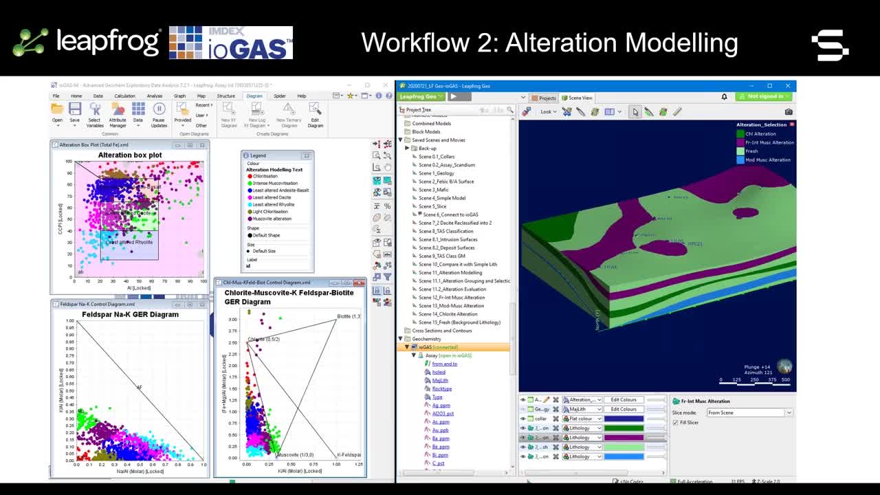
[00:38:12.740] is I’m going to open an alteration boxplot.
[00:38:18.450] So this sort of diagram, as you can see here,
[00:38:22.170] it consists of two axis
[00:38:24.180] the alteration index, Ishikawa Alteration Index,
[00:38:27.000] versus the chloride carbonate pyrite index or CCPI.
[00:38:31.180] So the alteration box plot was developed specifically
[00:38:34.650] for the study of alteration associated with VHMS systems.
[00:38:39.250] And even though it’s used for that purpose,
[00:38:40.940] and while they’re not certain that we are looking
[00:38:44.220] at a VMS deposit here,
[00:38:46.490] we can use the processes that are presented
[00:38:49.470] in this sort of diagram as a starting point.
[00:38:53.050] So by no means we should take the information that’s present
[00:38:56.470] in this as the gospel,
[00:39:00.825] or as a silver bullet, to let you know
[00:39:03.650] if you’re looking at this sort
[00:39:04.690] of alteration type, but it’s a good place
[00:39:07.400] to start, and why is it a good place to start?
[00:39:09.770] And it’s because in this diagram,
[00:39:12.700] which consists of the AI and CCPI axes.
[00:39:17.390] So the X axis represents a loss of sodium and calcium
[00:39:22.760] and gain of potassium and magnesium within this index.
[00:39:26.750] So that’s represented by the development of muscovite
[00:39:29.927] and chloride from alteration of sodic plagioclase.
[00:39:33.540] And Y axis CCPI is constructed
[00:39:36.262] in a way that it represents an increase
[00:39:39.080] of magnesium and FEO related to core development.
[00:39:42.960] So it allows you to separate out
[00:39:44.900] between muscovite and chloride development.
[00:39:47.360] And if you’re aware of that sort
[00:39:48.660] of processes, and the fact that we’ve labeled the nodes
[00:39:52.560] that corresponds to development of this mineral.
[00:39:54.710] So you can see on the right here,
[00:39:56.520] you have IL for elite, and you have here AB for albite
[00:40:00.520] and CHL at a top for chloride.
[00:40:03.110] So as long as you’re aware that this diagram represents
[00:40:06.320] the development of that assemblage of minerals,
[00:40:09.720] and you’re familiar and comfortable with that process,
[00:40:14.370] you’re able to use this sort of diagram to start thinking
[00:40:18.330] about how you can model alteration in your data.
[00:40:22.020] And the reason why I do this is because it’s a quick
[00:40:25.820] and easy way of coloring your data points automatically
[00:40:29.499] based on where they plot here.
[00:40:31.370] So if we find, we managed to find great success in coloring
[00:40:35.330] where the data points plot within the polygons here,
[00:40:38.090] because the data points that it plots
[00:40:39.730] within three boxes in the middle,
[00:40:42.380] they represent more fresh sort of composition.
[00:40:45.320] So and by fresh, I mean, less altered
[00:40:47.460] than the ones that’s outside of the box.
[00:40:49.930] And we can go one step further.
[00:40:52.150] And if we can assume that there’s little albite development
[00:40:56.120] or epidote sort of mineralization in this rocks.
[00:40:59.160] And basically what we can do is we can expand the field
[00:41:03.330] for the least altered rocks a bit more
[00:41:05.930] to the left hand side,
[00:41:09.550] and then we’re going to do the same thing
[00:41:13.210] with the middle box as well.
[00:41:14.390] So we just colored them up as dacite.
[00:41:19.619] So basically what we’re doing is we’re just expanding
[00:41:23.000] on the least altered classified blocks
[00:41:25.970] into a bigger classification,
[00:41:27.970] because we’re comfortable
[00:41:28.870] in knowing that the rocks had plots here,
[00:41:30.860] that they don’t represent any sort of alteration,
[00:41:32.990] even though they plot outside the least altered boxes.
[00:41:36.360] But we can call these guys
[00:41:39.950] some from hydrothermal alteration.
[00:41:41.950] And one thing to be really careful
[00:41:44.900] about in this is that there’s a certain risk
[00:41:48.820] in looking at this diagram on its own,
[00:41:51.220] because samples that plot higher up on the CCPI access,
[00:41:54.370] for example, because you’re looking
[00:41:56.330] at a ratio of magnesium plus iron over this elements.
[00:42:03.990] And because you’re looking at some mafic rocks in here.
[00:42:06.940] So if you remember just in the first workflow,
[00:42:09.770] we’ve actually identified
[00:42:11.170] that some of these rocks actually correspond
[00:42:12.890] to the basaltic composition.
[00:42:15.570] And what it means is that while it’s plotting up
[00:42:18.860] in a hydrothermally altered field,
[00:42:20.770] they may not represent hydrothermal alteration,
[00:42:24.990] they just represent a more mafic variant in your data point.
[00:42:29.330] So samples that actually represent more mafic composition
[00:42:33.610] with the higher FEO and magnesium amount.
[00:42:38.922] So what’s the takeaway here?
[00:42:41.000] The takeaway is that we recommend using this sort
[00:42:43.290] of diagram in conjunction with molar element ratio diagrams
[00:42:47.700] to identify processes more closely.
[00:42:50.370] What I’m going to do now is I’m going
[00:42:53.110] to just keep this open here
[00:42:55.520] and I’m going to open a general element ratio diagram.
[00:42:59.660] So I’m going to start with this ratio
[00:43:02.290] of sodium over aluminum versus potassium over aluminum.
[00:43:07.780] So if you’re not familiar with molar element ratio diagrams,
[00:43:12.380] basically if you remember stoichiometric composition
[00:43:17.490] of muscovite and all your feldspar minerals,
[00:43:21.980] you know that this sort
[00:43:23.560] of diagram represents that ratio of say
[00:43:29.935] sodium over aluminum and albite,
[00:43:32.260] and then ratio of say potassium
[00:43:34.170] to aluminum and muscovite which is 0.33.
[00:43:37.440] So you’re using the stoichiometric composition
[00:43:40.330] to define where the nodes,
[00:43:43.090] these dots sort of sit in this sort of diagram.
[00:43:45.613] And you’re able to use this
[00:43:48.050] in conjunction with our known composition in ioGAS.
[00:43:53.110] So what we provide within ioGAS
[00:43:55.380] is a way to plot say known composition
[00:43:58.740] of sheet silica stoichiometric composition.
[00:44:02.100] So you have an option of selecting from chloride
[00:44:04.900] and muscovite and all of your clay minerals composition here
[00:44:09.910] that would be familiar to you
[00:44:12.060] in this sort of alteration setting.
[00:44:14.980] So if we just turn everything on here
[00:44:19.955] and then seeing where they plot in this of diagram,
[00:44:23.595] and you can see that the muscovite node
[00:44:27.950] sort of sits here and here.
[00:44:29.800] So this is a way for you to basically see the processes
[00:44:33.440] that you would expect to see in a sort
[00:44:34.980] of rock soil, it’s overlapping here, but you basically,
[00:44:37.260] you have a bunch of chloride composition that sits here.
[00:44:40.280] So what can we tell basically from this diagram?
[00:44:44.250] Basically, we’re seeing
[00:44:46.910] how we can further subdivide the rocks
[00:44:50.423] that were logged as hydrothermal into a way
[00:44:58.915] that’s more easier to understand and more useful to us.
[00:45:03.270] And the way we’ve done that is we’ve created
[00:45:05.370] new color groups based on where they plot.
[00:45:07.540] So I’m just going to show you a very quick example
[00:45:10.260] before we move on, so I’m going to basically set everything
[00:45:16.048] to invisible except for the hydrothermal altered rocks.
[00:45:21.360] And then I’m going to create a new color group.
[00:45:31.400] Now I’m just going to create a new color group
[00:45:32.840] for intense muscovite alteration.
[00:45:35.100] And I’m going to label the rocks
[00:45:38.730] that are here as a new color group,
[00:45:41.820] and I’m going to create a new color group
[00:45:46.968] for chloride alteration.
[00:45:53.060] So this is a way for you to basically sub-divide
[00:45:58.040] your classification a bit more, right?
[00:46:01.256] And so I’ve done this process a bit manually before,
[00:46:04.760] so I’m just going to jump through,
[00:46:06.260] I’m just going to cheat a bit
[00:46:07.980] and I’m going to author attribute by what I’ve done.
[00:46:11.780] And so basically,
[00:46:14.051] I’ve done this process over the entire dataset
[00:46:18.410] just before this webinar,
[00:46:20.150] but basically this is the shortcut that I did
[00:46:22.110] ’cause I’ve already done this.
[00:46:23.177] So the sort of process involved was knowing
[00:46:26.470] that you’re looking at a range
[00:46:29.090] of alteration from sodium plagioclase to a more,
[00:46:33.295] your sodium plagioclase composition
[00:46:36.210] would plot somewhere here.
[00:46:37.660] And then you would see a pattern
[00:46:38.820] that leads them to be more altered towards here.
[00:46:41.860] And you see a development of chloride here.
[00:46:43.970] And you see sort of like the in-between zone
[00:46:46.550] so with the slight muscovite alteration,
[00:46:49.030] as opposed to intense muscovite alteration
[00:46:51.720] and slight colorization, sort of like that halfway point
[00:46:55.530] between more fresh composition and this one.
[00:46:59.050] And it’s important to know exactly
[00:47:01.880] what processes that you’re looking at
[00:47:04.400] because as I’ve tried to do here
[00:47:06.560] is I have managed to redefine the alteration process
[00:47:11.300] for the least altered ones.
[00:47:13.120] And you can see that the least altered rocks
[00:47:15.470] that are identified in the alteration boxplot,
[00:47:19.350] that when you bring them up,
[00:47:22.390] that they actually belong in three boxes,
[00:47:25.760] and that’s why they’re resulting in three color groups
[00:47:29.790] and because of that, they were presented
[00:47:31.910] in our fairing CCPI amount
[00:47:33.740] because of that mafic to felsic gradient.
[00:47:36.900] And it’s also represented to some extent in the X axis here.
[00:47:40.640] So it’s important to know the processes
[00:47:42.403] that you’re looking at and by applying large scale
[00:47:46.210] sort of alteration modeling to this
[00:47:48.890] based on the mineralogy of what you’re expecting to see.
[00:47:52.600] And I’m plotting them up as color groups
[00:47:55.595] within ioGAS, and then sub-dividing it as such based
[00:47:59.105] on your known, the minerals that you would expect to see,
[00:48:01.565] and then just doing the same as before.
[00:48:03.630] So just creating a new color group based on this.
[00:48:08.850] And I didn’t show this in the first workflow,
[00:48:09.947] but I’m just going to do it now.
[00:48:12.360] So I’m going to create a new color group
[00:48:14.000] and that’s going to be created
[00:48:15.910] as a new text column within ioGAS
[00:48:17.790] and within Leapfrog Geo, it’s going
[00:48:19.710] to be reflected under the assay tab once that’s done.
[00:48:23.430] And basically that allows you to create alteration model
[00:48:28.800] within Leapfrog Geo.
[00:48:30.420] And just one thing before we proceed.
[00:48:35.180] So just while on that subject,
[00:48:38.440] the alteration boxplot, the total FE alteration boxplot.
[00:48:42.640] You see that your at least altered rocks are plotting
[00:48:44.890] in the three boxes in the middle.
[00:48:46.700] And this is why it’s important
[00:48:49.205] to know that you will need
[00:48:50.440] to always look at this, not just on their own.
[00:48:54.940] So you’ll need to know why they’re different on the Y axis.
[00:48:59.910] And if you plot up your CCPI versus your SIO2 value,
[00:49:05.100] what’s actually interesting
[00:49:08.950] is that it varies with the silica
[00:49:12.310] that you’re looking at here.
[00:49:14.890] So it’s important to know
[00:49:16.900] that the variation in your CCPI is actually controlled,
[00:49:20.180] not just from the value
[00:49:22.260] of the numerator and denominator of the index,
[00:49:26.470] but also by other elements that might affect that as well.
[00:49:29.900] You’re looking at this
[00:49:30.840] in conjunction with your local lithology,
[00:49:36.150] or for example, by the task classification,
[00:49:40.860] you’re able to sort of see what’s actually happening here,
[00:49:44.320] so you can change the shape to the task classification
[00:49:48.530] that we did in workflow one,
[00:49:50.750] and you plot them with alteration modeling
[00:49:52.950] and you basically allow yourself
[00:49:55.310] to infer certain processes
[00:49:57.624] based on what you’ve already done so far.
[00:49:59.530] So it’s important not
[00:50:00.620] to just look at these diagrams on their own
[00:50:03.700] or these plots on their own, but using the various tools
[00:50:07.895] that we have in ioGAS, looking at them in conjunction
[00:50:10.110] with one another, to reach a certain conclusion,
[00:50:13.030] and that is the alteration modeling that we came up with.
[00:50:16.570] As that’s already being like back flagged into Leapfrog Geo
[00:50:20.270] as a new column under the assay table here,
[00:50:25.190] Allan can create a new geology model
[00:50:27.910] based on this new back flag information.
[00:50:30.310] So over to you Allan, thank you.
[00:50:32.653] <encoded_tag_open />v Allan<encoded_tag_closed />Thank you Putra.<encoded_tag_open />/v<encoded_tag_closed />
[00:50:33.610] Back to Leapfrog Geo.
[00:50:35.990] This is where you can find the back flag alteration modeling
[00:50:40.870] in Leapfrog Geo, so I’m just going to highlight,
[00:50:43.320] just click on the edit colors menu in here.
[00:50:46.710] This is where you can see the chlorination occurs,
[00:50:51.900] intense muscovite alteration,
[00:50:54.930] and this are your less altered alteration.
[00:50:59.810] You’ve got light chloride alteration
[00:51:01.490] in here, and you also have the muscovite alteration.
[00:51:04.510] Just going to click okay.
[00:51:06.434] I got to go through back to my save scenes.
[00:51:10.220] First is in order to model this because the nature
[00:51:13.550] of the alteration is a bit layered complex as well.
[00:51:17.020] And what we need to do
[00:51:18.400] is a bit of a simplification to the alterations.
[00:51:22.900] So what I’ve done is I’ve grouped those lists out,
[00:51:27.730] it became fresh,
[00:51:29.390] and then from fresh to intense muscovite alteration
[00:51:33.190] as well is one group, the chloride alteration is one group,
[00:51:36.630] as well as the moderate muscovite alteration
[00:51:39.100] is also one group.
[00:51:40.870] So it’s going to show you this.
[00:51:44.710] This is now the model,
[00:51:46.850] the fresh to intense muscovite alteration.
[00:51:50.270] Secondly, I have the moderately muscovite alteration
[00:51:55.560] at the base of the fresh to intense muscovite alteration.
[00:52:00.220] And lastly, what you have
[00:52:01.750] in here is your chloride alteration.
[00:52:05.270] Generating the output volumes.
[00:52:08.080] We now have the fresh in the background as well.
[00:52:10.640] So again, due to the layering nature
[00:52:14.330] of both of the rocks and alteration, you can see
[00:52:17.200] in here, the alteration output volumes
[00:52:20.450] that was produced is also layered.
[00:52:24.470] Want to slice through on the alteration model now,
[00:52:30.130] just to gain a bit of
[00:52:32.050] an appreciation on how this looks like at various sections.
[00:52:44.080] So again, just to summarize this,
[00:52:46.970] we’ve generated this simple lithology first,
[00:52:50.370] which is displayed on the 3D scene and then
[00:52:57.350] we made a detailed rock classification
[00:52:59.750] on the simple lithology, and then lastly,
[00:53:03.145] we generated an alteration model out of that.
[00:53:07.860] So Leapfrog Geo is a workflow based
[00:53:10.010] 3D implicit geological modeling tool,
[00:53:12.190] which allows you to quickly construct models directly
[00:53:15.750] from various sources, including drill holes,
[00:53:18.880] points, and surfaces.
[00:53:21.960] So ioGAS is an exploratory data analysis software
[00:53:25.210] for the detection of patterns, anomalies,
[00:53:28.550] and relationships in your geochemical data.
[00:53:33.150] We can bring data from Leapfrog Geo
[00:53:36.295] to ioGAS, and then back to Leapfrog Geo
[00:53:38.310] through the ioGAS link in the form of points
[00:53:41.260] or interval data.
[00:53:44.118] And then lastly,
[00:53:45.620] rock alteration or mineralization classification
[00:53:48.880] can be established in ioGAS
[00:53:51.160] and viewed and modeled in the Leapfrog Geo.
[00:53:56.620] Thank you so much for your time.
[00:53:58.390] Do you have any questions at this stage?
[00:54:01.874] <encoded_tag_open />v Host<encoded_tag_closed />Hi, Allan and Putra, great presentation,<encoded_tag_open />/v<encoded_tag_closed />
[00:54:05.140] that was fantastic to see the workflows
[00:54:07.340] from Leapfrog to ioGAS and back to Leapfrog again.
[00:54:11.550] We do have a couple of questions from attendees online.
[00:54:16.590] The first question is for Putra,
[00:54:19.335] how can I just predict the type
[00:54:21.690] of mineralization within the dataset?
[00:54:25.000] <encoded_tag_open />v Putra<encoded_tag_closed />So ultimately that depends on what you’re trying<encoded_tag_open />/v<encoded_tag_closed />
[00:54:29.220] to achieve within ioGAS
[00:54:32.607] and it also depends on what data that you have.
[00:54:36.170] So if you’re looking at purely at geochemical data
[00:54:40.710] with some information about
[00:54:42.890] what interval corresponds to what sort of mineralization,
[00:54:46.100] you’re sort of halfway there in terms of determining
[00:54:50.235] what mineralization is present within your data.
[00:54:53.340] Generally, it’s a very GIS type approach
[00:54:56.110] in that the more, like the more you can be certain
[00:54:59.290] about the interpretation that you come up with.
[00:55:02.260] But also in terms of what we can do
[00:55:05.455] in ioGAS, our classification diagrams will allow you
[00:55:08.940] to see if you’re within the ballpark
[00:55:11.600] of a certain prospective rock type.
[00:55:14.610] So one of the diagrams that we came up with
[00:55:18.080] quite recently is a Scott Haley diagram,
[00:55:21.850] just using a ratio of a couple of immobile elements
[00:55:25.570] in porphyry exploration.
[00:55:27.720] So that’s looking at a ratio
[00:55:29.995] of vanadium over scandium versus scandium.
[00:55:33.890] And that’s a really good way of determining if your data
[00:55:37.730] is situated within perspective porphyry copper field.
[00:55:42.200] So that’s just one example.
[00:55:44.470] And as I was showing in the presentation,
[00:55:46.160] we have a library of mineral composition
[00:55:50.710] and composition of known deposits, famous deposits.
[00:55:56.720] So those are the ones that Carl Brohart collated
[00:56:00.500] in his Austin ACA dataset,
[00:56:03.610] which we have implemented into ioGAS as a library.
[00:56:07.760] So it’s a library of known composition of type deposits,
[00:56:11.090] so famous deposits within certain deposit types.
[00:56:14.310] So say if you, for example,
[00:56:15.410] you’re exploring for IOCG type deposit and you have a sample
[00:56:20.700] that you think would be within the ballpark
[00:56:23.370] of let’s say an Olympic type deposit,
[00:56:27.680] and you can check if your data
[00:56:30.180] is plotting within that ballpark, within that range.
[00:56:33.790] So that’s one way of looking at it.
[00:56:35.510] But it’s always a good idea to have more info,
[00:56:39.620] so you plot your geochemical data
[00:56:43.830] in diagrams in ioGAS and you display out information,
[00:56:47.830] such as rock type and that sort of thing.
[00:56:50.250] If we have time, I might be able to share my screen
[00:56:54.440] and just show a few other things,
[00:56:56.970] but we’ll leave it up to another couple
[00:57:00.340] of questions before doing that, if that all right.
[00:57:02.930] <encoded_tag_open />v Host<encoded_tag_closed />Thanks Putra, great answer.<encoded_tag_open />/v<encoded_tag_closed />
[00:57:05.170] This next question is for Allan.
[00:57:07.970] So can I use point data such as my surface samples
[00:57:11.960] in the same workflow that you just presented today?
[00:57:15.750] <encoded_tag_open />v Allan<encoded_tag_closed />Thank you so much<encoded_tag_open />/v<encoded_tag_closed />
[00:57:16.988] for the question, very interesting question.
[00:57:18.990] So yes, you can.
[00:57:20.360] So if you have surface samples
[00:57:22.120] with multi-element geochemistry,
[00:57:24.510] similar to what we have in the drill holes.
[00:57:26.800] So you can use this.
[00:57:28.630] Actually, I’ve dealt with a previous project
[00:57:32.960] from one of our clients, and they’ve got soil samples
[00:57:38.020] and we have their multi elementary chemistry,
[00:57:40.670] and we were able to determine perspective areas
[00:57:45.080] through that particular data.
[00:57:47.720] <encoded_tag_open />v Host<encoded_tag_closed />Thanks, Allan.<encoded_tag_open />/v<encoded_tag_closed />
[00:57:49.320] Next question is for Putra,
[00:57:51.680] is there a recommendation you have
[00:57:53.240] for the number of elements required for workflow like this,
[00:57:56.810] do we need 33 as in the example that you used today?
[00:58:02.000] <encoded_tag_open />v Putra<encoded_tag_closed />So look in terms of elements,<encoded_tag_open />/v<encoded_tag_closed />
[00:58:03.870] it’s really not how much elements you have analyzed,
[00:58:07.990] even though that could be nice,
[00:58:09.610] but it’s also how they’re analyzed,
[00:58:12.790] and with the certain analytical methods that’s required
[00:58:16.520] to get the best out of your data.
[00:58:19.370] I guess the answer to that is pretty broad,
[00:58:22.155] but having a full list of 33 elements,
[00:58:29.500] having high quality, less of 20 something elements
[00:58:33.610] versus 60 element dataset,
[00:58:36.310] that’s analyze using the lowest cost analytical method.
[00:58:40.040] It might be better to go
[00:58:41.190] with ones that are more high quality.
[00:58:43.850] And I think it’s always good
[00:58:45.510] to emphasize that it’s preferable
[00:58:48.170] to know what you’re trying to look for,
[00:58:50.140] so what alteration assemblage,
[00:58:52.700] what lithology and what face of alteration
[00:58:57.400] or lithology that you’re expecting in your data
[00:59:00.830] and that sort of determines how many elements you need,
[00:59:03.800] what elements you need to look out for,
[00:59:06.020] and the quality that you want to seek
[00:59:09.450] in your data, because ultimately that will determine
[00:59:12.930] what sort of diagrams, classification diagrams,
[00:59:15.640] and what sort of advanced analytics tools
[00:59:18.600] that you can use in ioGAS.
[00:59:21.640] And of course, if you’re dealing
[00:59:22.940] with historical dataset
[00:59:24.220] as well, you have to bear in mind the sort
[00:59:28.648] of elements that will be advantages
[00:59:31.465] to compliment your historical dataset,
[00:59:34.460] if you’re not re-assaying them, for instance.
[00:59:38.070] So just that sort of thing will be need to keep in mind.
[00:59:43.134] So that’s a long winded answer
[00:59:44.680] to your question, but the short answer is 33 elements,
[00:59:48.800] as long as they’re of good quality,
[00:59:50.440] then you can go far with that, or even less,
[00:59:54.670] especially if they’re of high quality and they’re useful
[00:59:57.410] for the sort of thing you’re looking for.
[01:00:01.490] <encoded_tag_open />v Host<encoded_tag_closed />Awesome, thanks Putra.<encoded_tag_open />/v<encoded_tag_closed />
[01:00:02.860] I have another question here.
[01:00:05.180] What do you find are the most effective alteration tools
[01:00:08.420] when working with meta sediments,
[01:00:10.710] so if you have things like detrital silicates?
[01:00:13.963] That question is for Putra.
[01:00:15.950] <encoded_tag_open />v Putra<encoded_tag_closed />So when you’re looking at detrital silicates,<encoded_tag_open />/v<encoded_tag_closed />
[01:00:18.980] we don’t have a particular diagram that’ll be quite useful
[01:00:23.250] so that even though we have a bit of sort of like
[01:00:27.480] some more weathering trend sort of alteration diagrams.
[01:00:31.690] So if you’re familiar with the ACNK sort of diagram,
[01:00:37.575] they may be useful for what you’re trying to achieve,
[01:00:40.410] but ultimately I think
[01:00:42.313] if you’re working with meta sediments
[01:00:44.820] and looking at, which include detrital silicates,
[01:00:48.100] you probably will do well with just plotting them up
[01:00:51.700] in a few scatterplots, in ioGAS and using a combination
[01:00:55.630] of weathering trend alteration diagrams within ioGAS,
[01:00:59.110] so within that folder and just exploring what sort
[01:01:01.660] of works with your data and seeing if things are plotting
[01:01:04.120] where you expect them to be.
[01:01:06.280] <encoded_tag_open />v Host<encoded_tag_closed />Awesome, thanks Putra.<encoded_tag_open />/v<encoded_tag_closed />
[01:01:07.133] So this is question based on your experience,
[01:01:10.070] for both Allan and Putra,
[01:01:12.110] that if you had different classifications
[01:01:14.140] based on lithology and geochemistry,
[01:01:16.590] like we saw a little bit in today’s workflow,
[01:01:19.490] what are your best options for evaluating
[01:01:21.700] which classification has more confidence?
[01:01:25.540] <encoded_tag_open />v Putra<encoded_tag_closed />So I can start with this one, Allan.<encoded_tag_open />/v<encoded_tag_closed />
[01:01:27.780] So I guess based on next experience,
[01:01:29.220] just if you’re looking at just purely geochemical data,
[01:01:34.620] and if you’re trying to reconcile
[01:01:36.795] between what one diagram says and what your geology says,
[01:01:40.940] it’s always a good idea to step outside the circle
[01:01:43.860] and sort of think outside the box
[01:01:45.610] on what sort of other data that you can put in.
[01:01:49.810] And even though it doesn’t directly answer your question,
[01:01:51.630] but it’s always a good idea
[01:01:53.900] to add things like the spectral data
[01:01:57.120] from Osiris for example, and if you use that in conjunction
[01:02:00.360] with the workload that we presented here today,
[01:02:02.350] to be more certain of what you’re looking for,
[01:02:06.130] because ultimately, what we presented here today,
[01:02:09.010] so for example with the sodium
[01:02:11.489] over aluminum versus potassium over aluminum
[01:02:14.870] molar element ratio diagram,
[01:02:16.640] it’s not a silver bullet to sort of
[01:02:20.050] indicate the sort of alteration that you will see.
[01:02:22.440] So for example, and as status said, there’s no information
[01:02:25.560] in the file was of alteration is present.
[01:02:28.260] If I can just quickly share my screen.
[01:02:30.440] So in ioGAS we’re able
[01:02:31.980] to basically display a label right next to each data point.
[01:02:40.330] Basically, if I can show item labels.
[01:02:43.360] So each of the rock type here
[01:02:45.640] in each of the data point has been logged visually
[01:02:48.370] in the field, so what I’ve classified as prioritize rocks,
[01:02:55.510] and when you zoom into these data points a bit,
[01:02:57.990] and you see how they’re classified
[01:03:00.715] in the field, chloretic mafic flow.
[01:03:02.620] So that’s what they’re classified
[01:03:04.170] as chloride carbonate altered basalt
[01:03:07.740] and chloride carbonate shears, chloride porphyry.
[01:03:13.580] So it’s this sort of thing
[01:03:15.480] where you’re reconciling your log alteration
[01:03:19.580] with the alteration modeling
[01:03:21.480] that you’ve identified through this sort of diagrams.
[01:03:23.920] And if you move up a bit
[01:03:25.320] into the sericite alteration field,
[01:03:27.330] you see that it’s quite consistent
[01:03:29.550] with what we’ve identified
[01:03:30.990] using our geochemical classification.
[01:03:33.100] So you got your sericite chloride quartz porphyry
[01:03:37.880] and sericite altered quartz porphyry again,
[01:03:40.740] and sericite quartz,
[01:03:42.500] and a few other samples that’s classified
[01:03:45.180] as sericite altered.
[01:03:46.900] So if you want to be certain
[01:03:49.170] that you’re looking at the same thing,
[01:03:51.890] it’s always a good idea to first bring it back
[01:03:54.840] to your geology, so that’s number one.
[01:03:57.590] And number two is you want to use a combination
[01:04:01.630] of not just one molar element ratio.
[01:04:05.910] So say you can also plot things up
[01:04:07.980] in a chloride molar element ratio diagram.
[01:04:12.310] So this is a way to separate out
[01:04:15.380] between your muscovite from chloride alteration.
[01:04:18.180] And you can see that in a tie line
[01:04:19.710] between muscovite and chloride you have some samples
[01:04:22.300] to exhibit sort of that halfway point
[01:04:24.200] between chloride and muscovitic composition.
[01:04:27.740] And of course you can update this classification, right?
[01:04:31.210] So this is an interesting one.
[01:04:32.270] So you have a couple of samples here
[01:04:35.450] that’s classified as sericite chloride quartz porphyry,
[01:04:38.140] and chloride carbonate sericite,
[01:04:39.990] that’s sort of in a tie line between muscovite and chloride.
[01:04:43.410] And linking it back to log geology and using a combination
[01:04:46.800] of not just one molar element ratio diagram,
[01:04:50.160] but using multiple molar element ratio diagrams,
[01:04:52.910] you’re able to identify processes,
[01:04:55.970] and then you can refine your classification more
[01:04:58.250] and then seeing them being reflected
[01:05:00.100] in different geo and real-time
[01:05:01.650] and update your alteration modeling in real-time as well.
[01:05:05.320] So that’s how you can reconcile
[01:05:07.140] sort of your different classification that exist,
[01:05:10.210] but it’s always a good idea to not just use one diagram,
[01:05:13.080] just have to use multiple and use your best judgment.
[01:05:16.440] And ioGAS is easy to use
[01:05:19.510] in terms of applying colored groups and that sort of thing,
[01:05:23.060] which means what you interpret is reflected visually
[01:05:27.760] in real-time instantaneously, in fact.
[01:05:32.060] <encoded_tag_open />v Allan<encoded_tag_closed />Just adding to what Putra is saying,<encoded_tag_open />/v<encoded_tag_closed />
[01:05:35.450] you need to have at least the four ingredients
[01:05:38.460] in order to make your best judgment.
[01:05:42.930] The four Gs are actually your GIS data
[01:05:46.280] where it lies in 3D space.
[01:05:50.740] I need to consider also the logging,
[01:05:54.830] the logging, the mapping, and also the geochem data as well.
[01:06:00.560] If you’ve got multi element and geochem data, sewer data
[01:06:04.860] as well, in terms of geophysics,
[01:06:09.067] you need to combine it with the magnetics, gravity, IP, EM.
[01:06:13.670] So aside from having robust geochemical data,
[01:06:18.810] you need to basically,
[01:06:21.030] in order to classify this more confidently,
[01:06:23.850] you need to combine this together
[01:06:25.130] with all the other ingredients such
[01:06:26.810] as geology, geophysics, and GIS data.
[01:06:30.410] <encoded_tag_open />v Host<encoded_tag_closed />Thanks, Allen and Putra, those are great responses.<encoded_tag_open />/v<encoded_tag_closed />
[01:06:33.310] That’s all the questions we have time for today.
[01:06:36.320] <encoded_tag_open />v Putra<encoded_tag_closed />And lastly, if you want<encoded_tag_open />/v<encoded_tag_closed />
[01:06:37.260] to get in touch with the Seequent support team,
[01:06:41.110] please get in touch with us through [email protected],
[01:06:45.230] or if you want to get in touch with the ioGAS team,
[01:06:48.620] if you want to learn more about ioGAS, you can get
[01:06:51.420] in touch with them through their global help desk,
[01:06:55.210] which is under reflex.com/product/ioGAS.
[01:07:00.690] Again, thank you so much for your time.
[01:07:02.830] I hope to see you all soon again
[01:07:04.610] to our future technical Tuesday webinars.
[01:07:07.540] Thank you so much.
[01:07:09.280] <encoded_tag_open />v Allan<encoded_tag_closed />Thanks, everyone.<encoded_tag_open />/v<encoded_tag_closed />
<wpml_invalid_tag original=»PHA+» />

Технический вторник: Объединение литологии и геохимии при помощи рабочих процессов ioGAS и Leapfrog Geo

Обзор

Смотреть больше видео по запросу

Узнайте больше о решении Seequent для горнодобывающей промышленности

Расшифровка видеозаписи

Related